Getting Started with R and RMarkdown
Overview
Teaching: 75 min
Exercises: 30 minQuestions
What are R and R Studio?
What is R Markdown?
How do I format text in R Markdown?
How do I perform tasks with R and store information?
Objectives
To become oriented with R and R Studio.
To understand the difference between code chunks and markdown text.
To learn about functions and objects.
Contents
Why learn to program?
Share why you’re interested in learning how to code. > ## Solution: > There are lots of different reasons, including to perform data analysis and generate figures. I’m sure you have more specific reasons for why you’d like to learn! {: .solution} {: .challenge}
Introduction to R and RStudio
To perform exploratory analyses, we need the data we want to explore and a platform to analyze the data.
You already have the data. But what platform will we use to analyze the data? We have many options!
We could try to use a spreadsheet program like Microsoft Excel or Google sheets that have limited access, less flexibility, and don’t easily allow for things that are critical to “reproducible” research, like easily sharing the steps used to explore and make changes to the original data.
We could also use a program like SAS or STATA, which are used by many epidemiologists. However, these programs are not freely available, the graphics are not as customizable, and there are not a ton of specialized packages for different niche analyses.
Instead, we’ll use a more general programming language to test our hypothesis. Today we will use R, but we could have also used Python for the same reasons we chose R. Both R and Python are freely available, the instructions you use to do the analysis are easily shared, and by using reproducible practices, it’s straightforward to add more data or to change settings like colors or the size of a plotting symbol.
Bonus: But why R and not Python?
There’s no great reason. Although there are subtle differences between the languages, it’s ultimately a matter of personal preference. Both are powerful and popular languages that have very well developed and welcoming communities of scientists that use them. As you learn more about R, you may find things that are annoying in R that aren’t so annoying in Python; the same could be said of learning Python. If the community you work in uses R, then you’re in the right place.
To run R, all you really need is the R program, which is available for computers running the Windows, Mac OS X, or Linux operating systems. You installed R while getting set up for this workshop.
To make your life in R easier, there is a great (and free!) program called RStudio that you also installed and used during set up. As we work today, we’ll use features that are available in RStudio for writing and running code, managing projects, installing packages, getting help, and much more. It is important to remember that R and RStudio are different, but complementary programs. You need R to use RStudio.
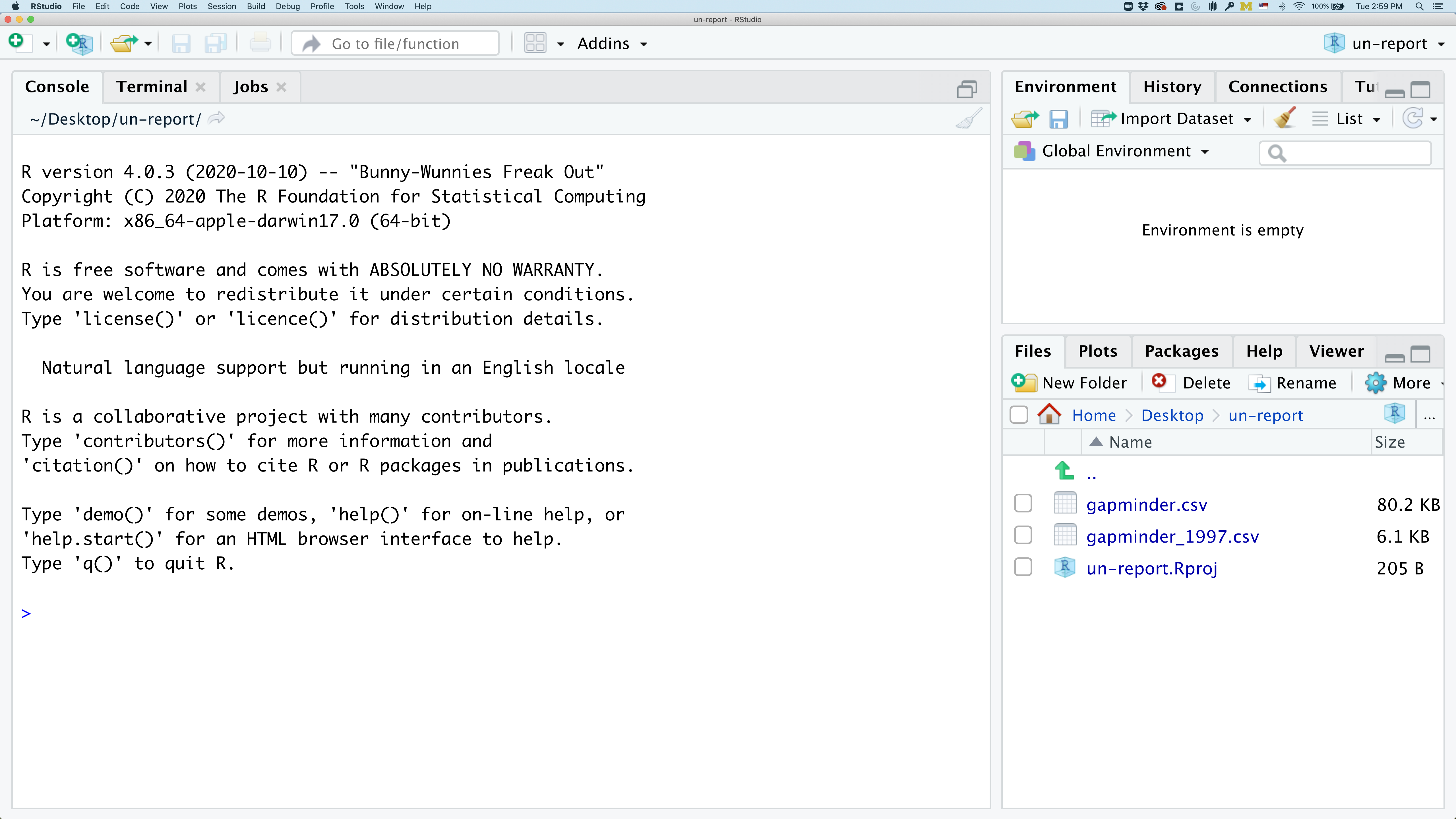
To get started, we’ll spend a little time getting familiar with the RStudio environment and setting it up to suit your tastes. When you start RStudio, you’ll have three panels.

On the left you’ll have a panel with three tabs - Console, Terminal, and
Jobs. The Console tab is what running R from the command line looks
like. This is where you can enter R code. Try typing in 2+2 at the
prompt (>).
In the upper right panel are tabs indicating the Environment, History, and a few other things. In the lower right panel are tabs for Files, Plots, Packages, Help, and Viewer. We’ll spend more time in each of these tabs as we go through the workshop, so we won’t spend a lot of time discussing them now.
Let’s get going on our analysis!
One of the helpful features in RStudio is the ability to create a project. A project is a special directory that contains all of the code and data that you will need to run an analysis.
At the top of your screen you’ll see the “File” menu. Select that menu and then the menu for “New Project…”.

When the smaller window opens, select “Existing Directory” and then the “Browse” button in the next window.
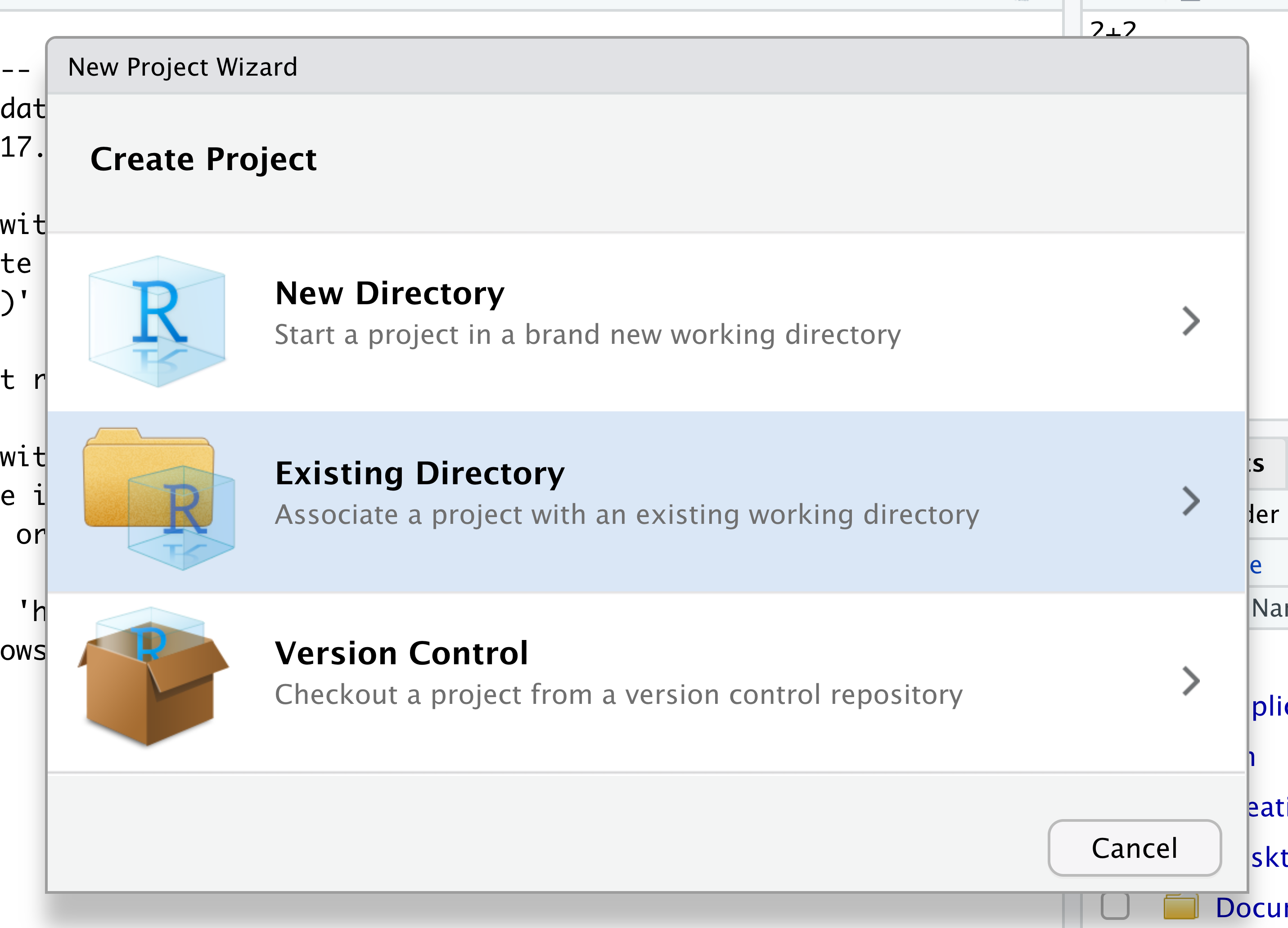

Navigate to the directory that contains your code and data from the setup instructions and click the “Open” button.
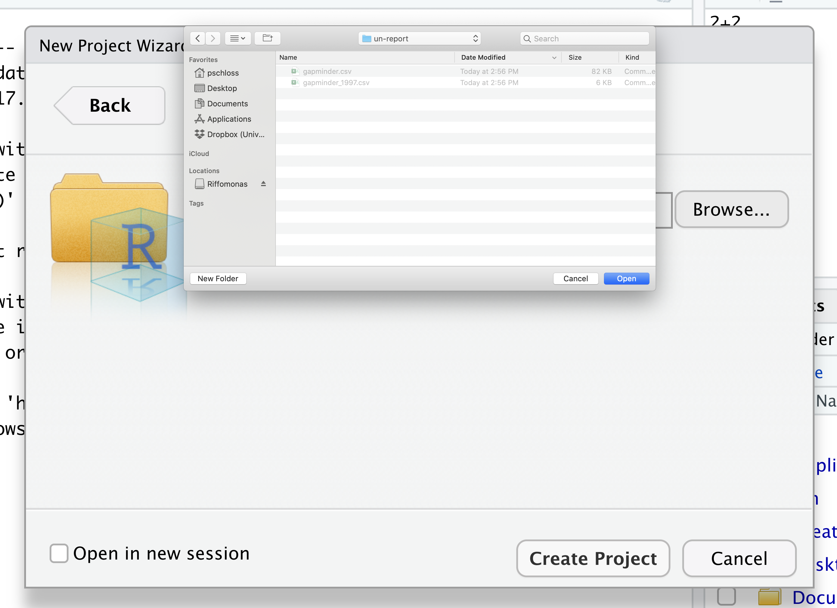
Then click the “Create Project” button.

Did you notice anything change?
In the lower right corner of your RStudio session, you should notice that your Files tab is now your project directory. You’ll also see a file called un-report.Rproj in that directory.
From now on, you should start RStudio by double clicking on that file. This will make sure you are in the correct directory when you run your analysis.
Introduction to R Markdown
We’d like to create a file where we can keep track of our R code.
Back in the “File” menu, you’ll see the first option is “New File”. Selecting “New File” opens another menu to the right and the fifth option is “R Markdown”. Select “R Markdown”.
Now we have a fourth panel in the upper left corner of RStudio that
includes an Editor tab with an untitled R Markdown file. Let’s save
this file as intro_to_r.Rmd in our project directory.
Why do we use R Markdown?
- It allows us to develop fully reproducible documents that weave together narrative text and code to produce formatted output.
- You can use it to generate a file in a format (html, word, pdf) that anybody can open and read, even without expertise in R. This is especially great for reporting results to mentors, advisors, PIs, bosses.
- You can keep a snapshot of your code to go back to if you run into issues later on down the line.
Components of an RMarkdown document
Below is what appears when you start a new .Rmd file:
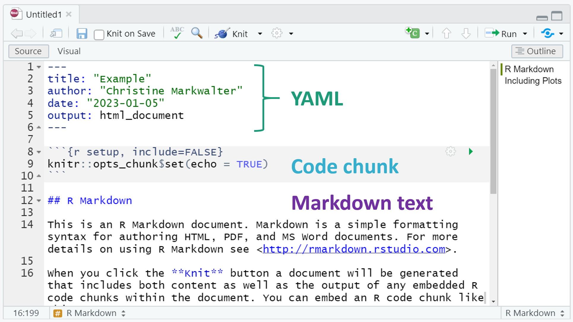
As you can see, there are three basic components: YAML, Markdown text, and R code chunks. These will work together to create your document output. In this course, we will output .html files.
YAML
YAML: sets the title, date, and output type. There are opportunities here for customization that we won’t cover in this course.
Markdown text
Markdown text: This is the narrative of the document that produces inline text in the .html output. There are many formatting opportunities here. The R Markdown cheat sheet is really helpful, but here are a few basics:
-
Single underscores (
_text_) or asterisks (*text*) produce italics -
Double underscores (
__text__) or asterisks (**text**) produce bold -
To create a bulleted list in R Markdown, you can use the
-(dash) or the*(asterisk). To add sub-bullets, hitTabbefore your dash or asterisk.
* This is a bullet
  * This is a sub-bullet
- This is also a bullet
  - This is also a sub-bullet
- Numbered lists can be generated similarly. If you’re not sure how
many items or what order you’d like them to be in, you can just make
them all
1., and markdown will be smart enough to number them in order.
1. This is my first point
1. I would also like to make this point
1. And finally, my last point
- Headers can be added using the
#symbol with a space afterwards. Sub-headings can be made for different levels by adding#symbols.
# This is a heading
## Sub heading
### Sub sub heading
#### Sub sub sub heading
Code chunks
Sections of the document that are dedicated to running R code are called “chunks.” This is where you will load packages, import, transform, and analyze data, and generate visualizations. It can be helpful to divide your work into many small chunks to help organize your code and focus any debugging.
All code chunks start with three back-ticks and curly brackets that
contain parameters for the chunk ({}) and end with three more
back-ticks. You add your code between these lines. If you’d like to add
comments to your code, you do so the same way you would in a script
using the #.
You can add a code chunk by typing it out, clicking the green icon at the top of the script editor, or using the keyboard shortcuts Ctrl + Alt + i.
Within the curly brackets, you can tell R what you want it to do with the code. Here’s a summary of options:
- For an R Markdown document, they will always start with
rto indicate that the language in the code chunk is R. - You can name a chunk (eg
{r loading_packages}), which can help organize your work. Every chunk MUST have a unique name. - Other arguments can impact how the code and output are evaluated
and/or displayed:
eval = FALSEdoes not run the codeecho = FALSEdoes not print the chunk’s R source code in the output document (though the output IS printed)warning = FALSEdoes not print warnings produced by R codemessage = FALSEdoes not print any messages producedinclude = FALSEdoes not include the chunk at all in the output document
- These parameters can also be adjusted using the settings button at the top of a code chunk.
Important to know: knit and working directory
There’s one other thing that we need to do before we get started with
our report. To render our documents into html format, we can “knit” them
in R Studio. Usually, R Markdown renders documents from the directory
where the document is saved (the location of the .Rmd file), but we
want it to render from the main project directory where our .Rproj
file is. This is because that’s where all of our relative paths are from
and it’s good practice to have all of your relative paths from the main
project directory. To change this default, click on the down arrow next
to the “Knit” button at the top left of R Studio, go to “Knit Directory”
and click “Project Directory”. Now it will assume all of your relative
paths for reading and writing files are from the un-report directory,
rather than the reports directory.
Now that we have that set up, let’s start on the report!
Comments
Sometimes you may want to write comments in your code to help you remember what your code is doing, but you don’t want R to think these comments are a part of the code you want to evaluate. That’s where comments come in! Anything after a
#symbol in your code will be ignored by R:# this is a comment
Foundational topics
Functions
Functions are built-in procedures that automate a task for you. You input arguments into a function and the function returns a value. We’ll go over a few math functions to get our feet wet.
You call a function in R by typing it’s name followed by opening then closing parenthesis. Each function has a purpose, which is often hinted at by the name of the function.
Let’s start with the sqrt() function.
Let’s try to run the function without anything inside the parenthesis.
sqrt()
Error in sqrt(): 0 arguments passed to 'sqrt' which requires 1
We get an error message. Don’t panic! Error messages pop up all the time, and can be super helpful in debugging code.
In this case, the message tells us zero arguments were passed to the
function, but we need to input at least one. Many functions, including
sqrt(), require additional pieces of information to do their job. We
call these additional values “arguments” or “parameters.” You pass
arguments to a function by placing values in between the
parenthesis. A function takes in these arguments and works behind the
scenes to output something we’re interested in.
For example, we want to provide a number to sqrt(), namely the number
we want the square root of:
sqrt(4)
[1] 2
Here, the input argument is 4, and the output is 2, just like we’d expect.
Now let’s do an example where we might not know the expected output:
sqrt(2)
[1] 1.414214
Great, now let’s move onto a slightly more complicated function. If we
want to round a number, we can use the round() function:
round(3.14159)
[1] 3
Why did this round to three? What if we want it to round to a different number of digits?
Pro-tip
Each function has a help page that documents what arguments the function expects and what value it will return. You can bring up the help page a few different ways. If you have typed the function name in the Editor windows, you can put your cursor on the function name and press F1 to open help page in the Help viewer in the lower right corner of RStudio. You can also type
?followed by the function name in the console.For example, try running
?roundin the console. A help page should pop up with information about what the function is used for and how to use it, as well as useful examples of the function in action. As you can see,round()has two arguments: the numeric input and the number of digits to round to.
We can use the digits argument in round() to change how many decimal
places are kept:
round(3.14159, digits = 2)
[1] 3.14
Sometimes it is helpful - or even necessary - to include the argument name, but often we can skip the argument name, if the argument values are passed in the order they are defined:
round(3.14159, 2)
[1] 3.14
Position of the arguments in functions
Which of the following lines of code will give you an output of 3.14? For the one(s) that don’t give you 3.14, what do they give you?
round(x = 3.1415)round(x = 3.1415, digits = 2)round(digits = 2, x = 3.1415)round(2, 3.1415)round(3.14159265, 2)Solution
- The 1st line will give you 3 because the default number of digits is 0.
- The 2nd and 3rd lines will give you the right answer because the arguments are named, and when you use names the order doesn’t matter.
- The 4th line will give you 2 because, since you didn’t name the arguments, x=2 and digits=3.1415.
- The 5th line will also give you the right answer because the arguments are in the correct order. {: .solution} {: .challenge}
Bonus Exercise: taking logarithms
Calculate the following: 1. Natural log (ln) of 10 1. Log base 10 of 10 (challenge: try to do this 2 different ways), and 1. Log base 3 of 10
Solution
# natural log (ln) of 10
log(10)
# log base 10 of 10
log10(10)
log(10, base = 10)
# log base 3 of 10
> log(10, base = 3)
{: .source} {: .solution} {: .challenge}
If all this function stuff sounds confusing, don’t worry! We’ll see a bunch of examples as we go that will make things clearer.
Objects
Sometimes we want to store information for later use or transformation. To do this in R, we store the information, or object, in a variable name that you can think of like a storage box.
Let’s say we want to round the square root of a number. One way we can do this is to put a function inside a function:
round(sqrt(2), 2)
[1] 1.41
Another way is to store the square root output first, and then round that.
To store an object for later, we first have to decide on a name of the
box we want to store it in. Let’s say we want to call it square_root.
Then we have to tell R what we want to put in the object name. We use
the <- symbol, which is the assignment operator to assign values
generated or typed on the right to object names on the left. An
alternative symbol that you might see used as an assignment operator
is the = but it is clearer to only use <- for assignment. We use
this symbol so often that RStudio has a keyboard short cut for it:
Alt+- on Windows, and
Option+- on Mac.
Let’s assign sqrt(2) to the object square_root. We can see that
square_root contains the square root of 2:
square_root <- sqrt(2)
square_root
[1] 1.414214
In R terms, square_root is a named object that references or
stores something. In this case, square_root stores the square root of
2.
Notice that we also have a new value in our environment in the upper right hand corner of RStudio. This panel lists all of the objects that we have stored in our environment, it’s kind of like a view into our storage room (environment) of all the boxes (objects) of things we have access to.
Now let’s round the square root of 2 to 2 decimal places:
sqrt_rounded <- round(square_root, 2)
sqrt_rounded
[1] 1.41
This is a fairly straightforward example, but you’ll see the usefulness of storing things in variables as the workshop progresses.
Now, what happens to sqrt_rounded if we update square_root?
square_root <- sqrt(4)
square_root
[1] 2
sqrt_rounded
[1] 1.41
It doesn’t update! That’s because we haven’t re-run the code that
rounded square_root. The values don’t update automatically like in a
spreadsheet.
Predicting object contents
What is
my_numberafter these three lines are run?my_number <- 10 my_number + 5 my_number <- my_number + 7
- 10
- 15
- 17
- 22
Solution
The answer is 17 because 10 is stored in
my_numberin the first line, 15 is printed after the second line but is not stored somy_numberremains 10, and then 7 is added tomy_numberin the third line, making 17. If we ran the third line again,my_numberwould be 24. Because the object value changes depending on the number of times we run the final line, in most cases it’s best practice to not overwrite objects like this. {: .source} {: .solution} {: .challenge}
Guidelines on naming objects
- They cannot start with a number (2x is not valid, but x2 is) or have special characters.
- R is case sensitive, so for example, weight is different from Weight.
- You cannot use spaces in the name.
- There are some names that cannot be used because they are the names of fundamental functions in R (e.g., if, else, for; see here for a complete list). If in doubt, check the help to see if the name is already in use (
?function_name). {: .checklist}
Bonus Exercise: Bad names for objects
Try to assign values to some new variable names. What do you notice? After running all four lines of code below, what value do you think the variable
Flowerholds?1number <- 3 Flower <- "marigold" flower <- "rose" favorite number <- 12Solution
Notice that we get an error when we try to assign values to
1numberandfavorite number. This is because we cannot start an object name with a numeral and we cannot have spaces in object names. The objectFlowerstill holds “marigold.” This is because R is case-sensitive, so runningflower <- "rose"does NOT change theFlowerobject. This can get confusing, and is why we generally avoid having objects with the same name and different capitalization. {: .solution} {: .challenge}
Getting unstuck
Sometimes you may accidentally run a line of code that isn’t quite complete yet. For instance:
my_number <-What happens when you run this? In your console at the bottom of your screen, you may see a
+instead of a>at the beginning of the line. This means that R is waiting for more information. In this case, it’s because it doesn’t know what you want to store inmy_number. You can do one of two things if this happens - finish the command you want to type (e.g. by entering a number), or hit the escape key to get unstuck. {: .callout}
Quotes vs. No Quotes
Let’s say we wanted to print out a word:
treeError: object 'tree' not foundYou’ll notice that we get an error, that the object ‘tree’ is not found. This is because R is looking for an object called
tree. But what we really want is to just print out the word “tree”. To do this, we put the word in quotes (single or double) so R knows that it’s not an object it needs to look for:"tree"[1] "tree"
Object structures
Objects may be a single piece of data like in the examples above, or they may consist of structured data. The image below (adapted from here ) shows some common data structures and their names.
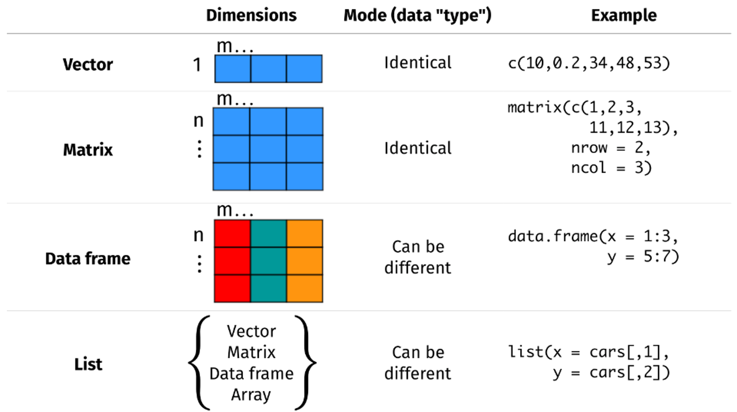
We will most commonly use Data Frames in this class. Note that Data Frames consist of variable vectors (columns) bound together that all have the same number of observations (rows).
Note that you can access individual vectors/columns within dataframes
using the $ symbol (eg dataframe$column)
Object classes
All objects stored in R have a class which tells R how to handle the object. In a data frame, different columns can be of different classes. Below are some of the most common classes:
| Class | Definition | Examples | Function to change class |
|---|---|---|---|
| Character | These are text/words/sentences “within quotation marks”. Math cannot be done on these objects. You may also hear these referred to as strings. | "Character objects are in quotation marks." |
as.character() |
| Numeric | These may be real or decimal numbers. | 3.14159, -3.14159, 100 |
as.numeric() |
| Factor | Used for categorical variables with an order or hierarchy of values. | Variable college_class with levels freshman, sophomore, junior, and senior. |
factor(levels = , labels = ) |
| Logical | Must be either TRUE or FALSE. |
TRUE or FALSE |
|
| Date | Once you tell R you are working with dates, you can manipulate and display them in specific ways. Note that the lubridate packages is ideal for handling dates. |
2023-01-13 |
Use the lubridate package |
Glossary of terms
- Comments: lines or parts of lines that are not run. In R, comments
start with a
#. - Function: takes input and generates output.
- Object: way to store information for later use and manipulation.
Key Points
R is a free programming language used by many for reproducible data analysis.
RMarkdown allows you to weave together narrative text and code.
Functions allow you to perform complex tasks.
Objects allow you to store information.