Introduction to The DiscovR Workshop
Overview
Teaching: 15 min
Exercises: 0 minQuestions
Who is the workshop for?
What will the workshop cover?
What else do I need to know about the workshop?
Objectives
Set expectations.
Meet each other.
Introduce the workshop goals.
Go over logistics.
DiscovR stands for “Data integration: strategies, concepts, and visuals in R”
Who is this workshop for?
This workshop is for data managers and others working with data who are interested in learning the foundations of data science and coding in R so you can use it in your own work. We believe everyone can learn to code, and that a lot of you will find it very useful for things such as data analysis and plotting.
This workshop is targeted to absolute beginners, and we expect that you have zero data science or coding experience coming in. That being said, you’re welcome to attend the workshop if you already have a coding background but want to learn more!
To provide an inclusive learning environment, we follow The Carpentries Code of Conduct. We expect that instructors, facilitators, and learners abide by this code of conduct, including practicing the following behaviors:
- Use welcoming and inclusive language.
- Be respectful of different viewpoints and experiences.
- Gracefully accept constructive criticism.
- Focus on what is best for the community.
- Show courtesy and respect towards other community members.
Introducing the instructors and facilitators
Now that you know a little about The Carpentries as an organization, the instructors and facilitators will introduce themselves and what they’ll be teaching/helping with.
Introducing participants
Introduce yourself with your preferred name, role, affiliation, work/research area, and Kenyan name and meaning.
What will the workshop cover?
This workshop will introduce you to exploratory data analysis and effective data visualiation, and how to implement these concepts using the R programming language.
While we will focus primarily on public health applications, what you learn here are programs that are used everyday in computational workflows in diverse fields: microbiology, statistics, neuroscience, genetics, the social and behavioral sciences, such as psychology, economics, and many others.
A workflow is a set of steps to read data, analyze it, and produce numerical and graphical results to support an assertion or hypothesis encapsulated into a set of computer files that can be run from scratch on the same data to obtain the same results. This is highly desirable in situations where the same work is done repeatedly – think of processing data from an annual survey. It is also desirable for reproducibility, which enables you and other people to look at what you did and produce the same results later on. It is increasingly common for people to publish scientific articles along with the data and computer code that generated the results discussed within them.
The programs we will use are:
- R: a statistical analysis and data management program,
- RStudio: a graphical interface to use R, and
- R Markdown: a method for writing reproducible reports.
We’ll use these tools to manage data, perform basic statistical analyses, and make pretty plots!
While the workshop won’t make you an expert, we hope to provide you with a foundational understanding in coding for data analysis and visualization, automating your work, and creating reproducible programs. We also hope to provide you with some fundamentals that you can incorporate in your own work.
At the end, we provide links to resources you can use to learn about these topics in more depth than this workshop can provide.
Asking questions and getting help
One last note before we get into the workshop.
If you have general questions about a topic, please raise your hand to ask it. The instructor will definitely be willing to answer!
For more specific nitty-gritty questions about issues you’re having individually, we use sticky notes to indicate whether you are on track or need help. We’ll use these throughout the workshop to help us determine when you need help with a specific issue (a facilitator will come help), whether our pace is too fast, and whether you are finished with exercises. If you indicate that you need help because, for instance, you get an error in your code (e.g. red sticky), a facilitator will come help you figure things out. Feel free to also call facilitators over through a hand wave if we don’t see your sticky!
Other miscellaneous things
If you’re in person, we’ll tell you where the bathrooms are! Also let us know if there are any accommodations we can provide to help make your learning experience better.
Key Points
We follow The Carpentries Code of Conduct.
Our fundamental goal is to become more comfortable exploring and working with data.
Our workshop goal is to write a sharable and reproducible report.
This lesson content is targeted to absolute beginners with no data science or coding experience.
Getting Started with R and RMarkdown
Overview
Teaching: 75 min
Exercises: 30 minQuestions
What are R and R Studio?
What is R Markdown?
How do I format text in R Markdown?
How do I perform tasks with R and store information?
Objectives
To become oriented with R and R Studio.
To understand the difference between code chunks and markdown text.
To learn about functions and objects.
Contents
Why learn to program?
Share why you’re interested in learning how to code. > ## Solution: > There are lots of different reasons, including to perform data analysis and generate figures. I’m sure you have more specific reasons for why you’d like to learn! {: .solution} {: .challenge}
Introduction to R and RStudio
To perform exploratory analyses, we need the data we want to explore and a platform to analyze the data.
You already have the data. But what platform will we use to analyze the data? We have many options!
We could try to use a spreadsheet program like Microsoft Excel or Google sheets that have limited access, less flexibility, and don’t easily allow for things that are critical to “reproducible” research, like easily sharing the steps used to explore and make changes to the original data.
We could also use a program like SAS or STATA, which are used by many epidemiologists. However, these programs are not freely available, the graphics are not as customizable, and there are not a ton of specialized packages for different niche analyses.
Instead, we’ll use a more general programming language to test our hypothesis. Today we will use R, but we could have also used Python for the same reasons we chose R. Both R and Python are freely available, the instructions you use to do the analysis are easily shared, and by using reproducible practices, it’s straightforward to add more data or to change settings like colors or the size of a plotting symbol.
Bonus: But why R and not Python?
There’s no great reason. Although there are subtle differences between the languages, it’s ultimately a matter of personal preference. Both are powerful and popular languages that have very well developed and welcoming communities of scientists that use them. As you learn more about R, you may find things that are annoying in R that aren’t so annoying in Python; the same could be said of learning Python. If the community you work in uses R, then you’re in the right place.
To run R, all you really need is the R program, which is available for computers running the Windows, Mac OS X, or Linux operating systems. You installed R while getting set up for this workshop.
To make your life in R easier, there is a great (and free!) program called RStudio that you also installed and used during set up. As we work today, we’ll use features that are available in RStudio for writing and running code, managing projects, installing packages, getting help, and much more. It is important to remember that R and RStudio are different, but complementary programs. You need R to use RStudio.
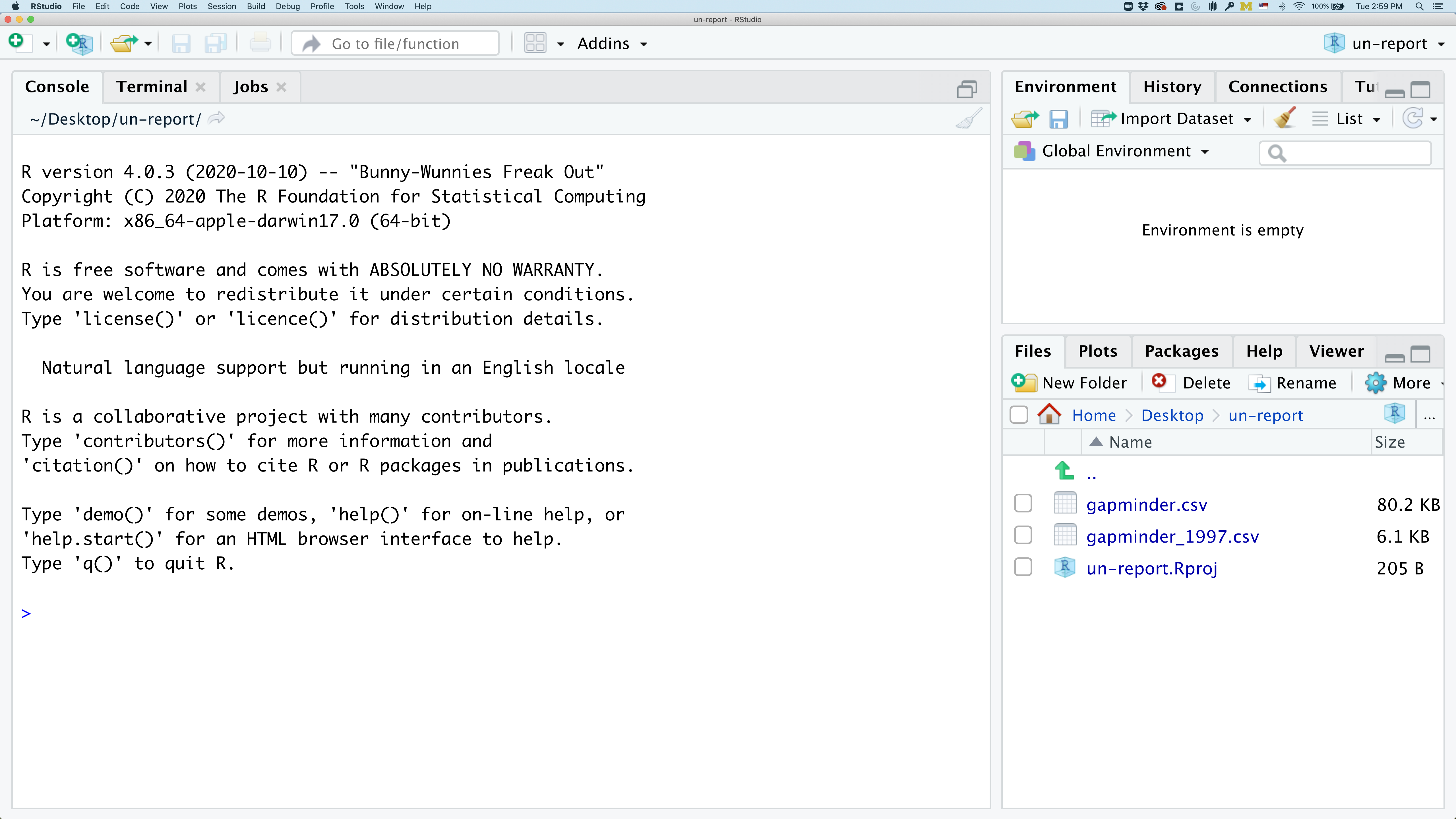
To get started, we’ll spend a little time getting familiar with the RStudio environment and setting it up to suit your tastes. When you start RStudio, you’ll have three panels.

On the left you’ll have a panel with three tabs - Console, Terminal, and
Jobs. The Console tab is what running R from the command line looks
like. This is where you can enter R code. Try typing in 2+2 at the
prompt (>).
In the upper right panel are tabs indicating the Environment, History, and a few other things. In the lower right panel are tabs for Files, Plots, Packages, Help, and Viewer. We’ll spend more time in each of these tabs as we go through the workshop, so we won’t spend a lot of time discussing them now.
Let’s get going on our analysis!
One of the helpful features in RStudio is the ability to create a project. A project is a special directory that contains all of the code and data that you will need to run an analysis.
At the top of your screen you’ll see the “File” menu. Select that menu and then the menu for “New Project…”.

When the smaller window opens, select “Existing Directory” and then the “Browse” button in the next window.
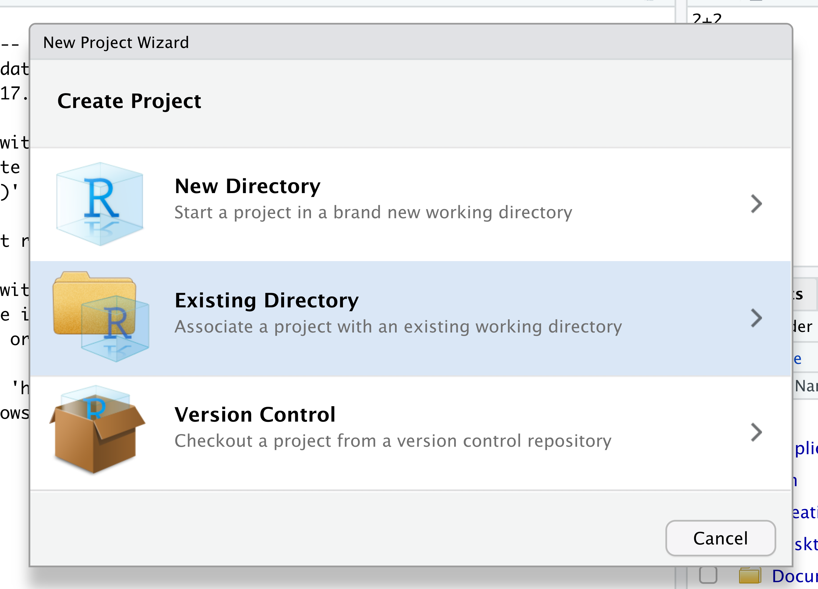

Navigate to the directory that contains your code and data from the setup instructions and click the “Open” button.
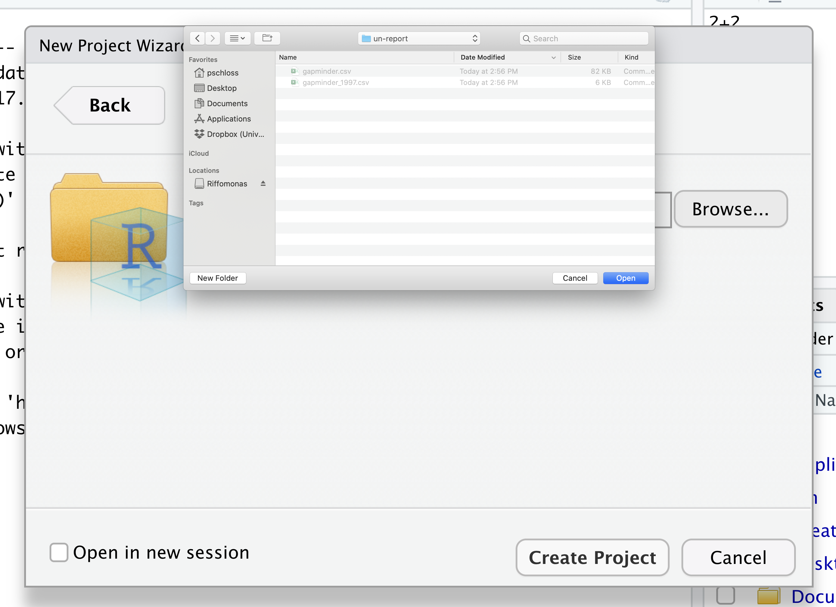
Then click the “Create Project” button.

Did you notice anything change?
In the lower right corner of your RStudio session, you should notice that your Files tab is now your project directory. You’ll also see a file called un-report.Rproj in that directory.
From now on, you should start RStudio by double clicking on that file. This will make sure you are in the correct directory when you run your analysis.
Introduction to R Markdown
We’d like to create a file where we can keep track of our R code.
Back in the “File” menu, you’ll see the first option is “New File”. Selecting “New File” opens another menu to the right and the fifth option is “R Markdown”. Select “R Markdown”.
Now we have a fourth panel in the upper left corner of RStudio that
includes an Editor tab with an untitled R Markdown file. Let’s save
this file as intro_to_r.Rmd in our project directory.
Why do we use R Markdown?
- It allows us to develop fully reproducible documents that weave together narrative text and code to produce formatted output.
- You can use it to generate a file in a format (html, word, pdf) that anybody can open and read, even without expertise in R. This is especially great for reporting results to mentors, advisors, PIs, bosses.
- You can keep a snapshot of your code to go back to if you run into issues later on down the line.
Components of an RMarkdown document
Below is what appears when you start a new .Rmd file:
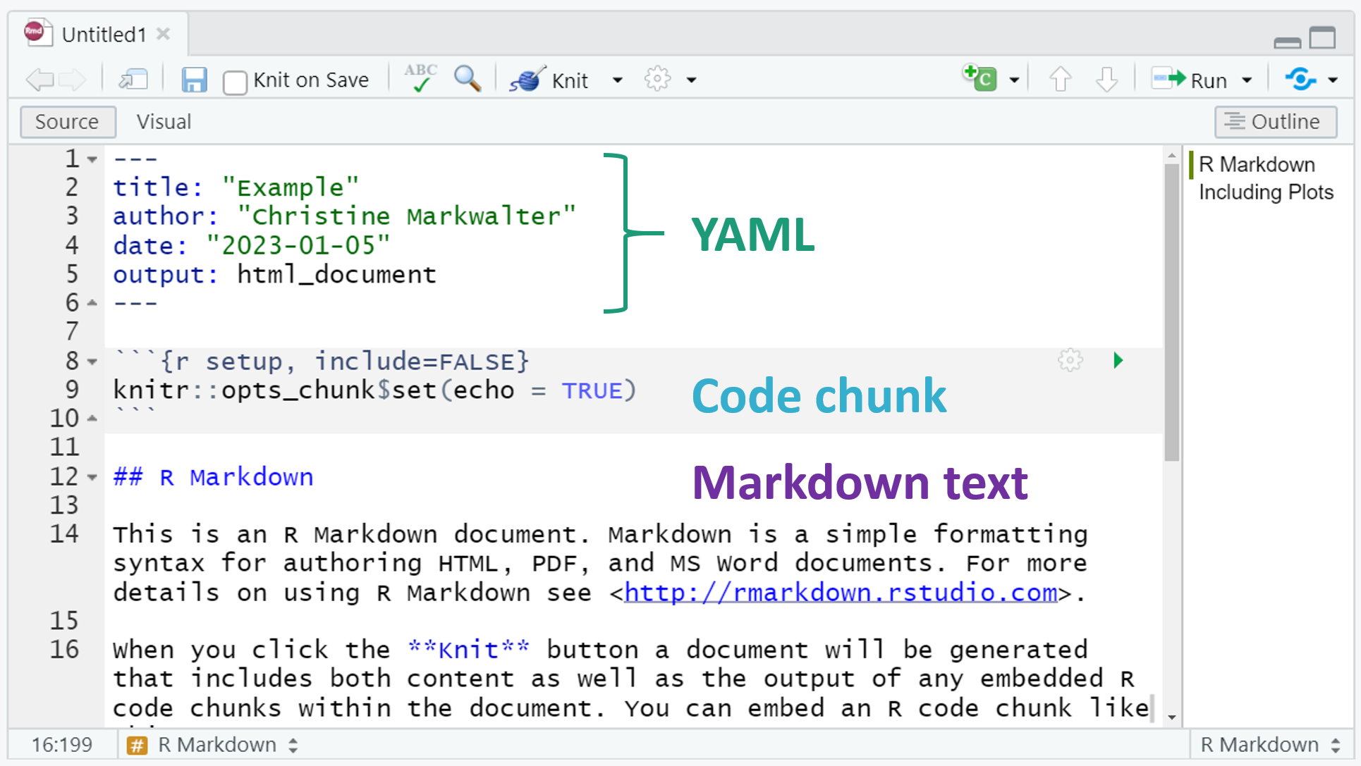
As you can see, there are three basic components: YAML, Markdown text, and R code chunks. These will work together to create your document output. In this course, we will output .html files.
YAML
YAML: sets the title, date, and output type. There are opportunities here for customization that we won’t cover in this course.
Markdown text
Markdown text: This is the narrative of the document that produces inline text in the .html output. There are many formatting opportunities here. The R Markdown cheat sheet is really helpful, but here are a few basics:
-
Single underscores (
_text_) or asterisks (*text*) produce italics -
Double underscores (
__text__) or asterisks (**text**) produce bold -
To create a bulleted list in R Markdown, you can use the
-(dash) or the*(asterisk). To add sub-bullets, hitTabbefore your dash or asterisk.
* This is a bullet
  * This is a sub-bullet
- This is also a bullet
  - This is also a sub-bullet
- Numbered lists can be generated similarly. If you’re not sure how
many items or what order you’d like them to be in, you can just make
them all
1., and markdown will be smart enough to number them in order.
1. This is my first point
1. I would also like to make this point
1. And finally, my last point
- Headers can be added using the
#symbol with a space afterwards. Sub-headings can be made for different levels by adding#symbols.
# This is a heading
## Sub heading
### Sub sub heading
#### Sub sub sub heading
Code chunks
Sections of the document that are dedicated to running R code are called “chunks.” This is where you will load packages, import, transform, and analyze data, and generate visualizations. It can be helpful to divide your work into many small chunks to help organize your code and focus any debugging.
All code chunks start with three back-ticks and curly brackets that
contain parameters for the chunk ({}) and end with three more
back-ticks. You add your code between these lines. If you’d like to add
comments to your code, you do so the same way you would in a script
using the #.
You can add a code chunk by typing it out, clicking the green icon at the top of the script editor, or using the keyboard shortcuts Ctrl + Alt + i.
Within the curly brackets, you can tell R what you want it to do with the code. Here’s a summary of options:
- For an R Markdown document, they will always start with
rto indicate that the language in the code chunk is R. - You can name a chunk (eg
{r loading_packages}), which can help organize your work. Every chunk MUST have a unique name. - Other arguments can impact how the code and output are evaluated
and/or displayed:
eval = FALSEdoes not run the codeecho = FALSEdoes not print the chunk’s R source code in the output document (though the output IS printed)warning = FALSEdoes not print warnings produced by R codemessage = FALSEdoes not print any messages producedinclude = FALSEdoes not include the chunk at all in the output document
- These parameters can also be adjusted using the settings button at the top of a code chunk.
Important to know: knit and working directory
There’s one other thing that we need to do before we get started with
our report. To render our documents into html format, we can “knit” them
in R Studio. Usually, R Markdown renders documents from the directory
where the document is saved (the location of the .Rmd file), but we
want it to render from the main project directory where our .Rproj
file is. This is because that’s where all of our relative paths are from
and it’s good practice to have all of your relative paths from the main
project directory. To change this default, click on the down arrow next
to the “Knit” button at the top left of R Studio, go to “Knit Directory”
and click “Project Directory”. Now it will assume all of your relative
paths for reading and writing files are from the un-report directory,
rather than the reports directory.
Now that we have that set up, let’s start on the report!
Comments
Sometimes you may want to write comments in your code to help you remember what your code is doing, but you don’t want R to think these comments are a part of the code you want to evaluate. That’s where comments come in! Anything after a
#symbol in your code will be ignored by R:# this is a comment
Foundational topics
Functions
Functions are built-in procedures that automate a task for you. You input arguments into a function and the function returns a value. We’ll go over a few math functions to get our feet wet.
You call a function in R by typing it’s name followed by opening then closing parenthesis. Each function has a purpose, which is often hinted at by the name of the function.
Let’s start with the sqrt() function.
Let’s try to run the function without anything inside the parenthesis.
sqrt()
Error in sqrt(): 0 arguments passed to 'sqrt' which requires 1
We get an error message. Don’t panic! Error messages pop up all the time, and can be super helpful in debugging code.
In this case, the message tells us zero arguments were passed to the
function, but we need to input at least one. Many functions, including
sqrt(), require additional pieces of information to do their job. We
call these additional values “arguments” or “parameters.” You pass
arguments to a function by placing values in between the
parenthesis. A function takes in these arguments and works behind the
scenes to output something we’re interested in.
For example, we want to provide a number to sqrt(), namely the number
we want the square root of:
sqrt(4)
[1] 2
Here, the input argument is 4, and the output is 2, just like we’d expect.
Now let’s do an example where we might not know the expected output:
sqrt(2)
[1] 1.414214
Great, now let’s move onto a slightly more complicated function. If we
want to round a number, we can use the round() function:
round(3.14159)
[1] 3
Why did this round to three? What if we want it to round to a different number of digits?
Pro-tip
Each function has a help page that documents what arguments the function expects and what value it will return. You can bring up the help page a few different ways. If you have typed the function name in the Editor windows, you can put your cursor on the function name and press F1 to open help page in the Help viewer in the lower right corner of RStudio. You can also type
?followed by the function name in the console.For example, try running
?roundin the console. A help page should pop up with information about what the function is used for and how to use it, as well as useful examples of the function in action. As you can see,round()has two arguments: the numeric input and the number of digits to round to.
We can use the digits argument in round() to change how many decimal
places are kept:
round(3.14159, digits = 2)
[1] 3.14
Sometimes it is helpful - or even necessary - to include the argument name, but often we can skip the argument name, if the argument values are passed in the order they are defined:
round(3.14159, 2)
[1] 3.14
Position of the arguments in functions
Which of the following lines of code will give you an output of 3.14? For the one(s) that don’t give you 3.14, what do they give you?
round(x = 3.1415)round(x = 3.1415, digits = 2)round(digits = 2, x = 3.1415)round(2, 3.1415)round(3.14159265, 2)Solution
- The 1st line will give you 3 because the default number of digits is 0.
- The 2nd and 3rd lines will give you the right answer because the arguments are named, and when you use names the order doesn’t matter.
- The 4th line will give you 2 because, since you didn’t name the arguments, x=2 and digits=3.1415.
- The 5th line will also give you the right answer because the arguments are in the correct order. {: .solution} {: .challenge}
Bonus Exercise: taking logarithms
Calculate the following: 1. Natural log (ln) of 10 1. Log base 10 of 10 (challenge: try to do this 2 different ways), and 1. Log base 3 of 10
Solution
# natural log (ln) of 10
log(10)
# log base 10 of 10
log10(10)
log(10, base = 10)
# log base 3 of 10
> log(10, base = 3)
{: .source} {: .solution} {: .challenge}
If all this function stuff sounds confusing, don’t worry! We’ll see a bunch of examples as we go that will make things clearer.
Objects
Sometimes we want to store information for later use or transformation. To do this in R, we store the information, or object, in a variable name that you can think of like a storage box.
Let’s say we want to round the square root of a number. One way we can do this is to put a function inside a function:
round(sqrt(2), 2)
[1] 1.41
Another way is to store the square root output first, and then round that.
To store an object for later, we first have to decide on a name of the
box we want to store it in. Let’s say we want to call it square_root.
Then we have to tell R what we want to put in the object name. We use
the <- symbol, which is the assignment operator to assign values
generated or typed on the right to object names on the left. An
alternative symbol that you might see used as an assignment operator
is the = but it is clearer to only use <- for assignment. We use
this symbol so often that RStudio has a keyboard short cut for it:
Alt+- on Windows, and
Option+- on Mac.
Let’s assign sqrt(2) to the object square_root. We can see that
square_root contains the square root of 2:
square_root <- sqrt(2)
square_root
[1] 1.414214
In R terms, square_root is a named object that references or
stores something. In this case, square_root stores the square root of
2.
Notice that we also have a new value in our environment in the upper right hand corner of RStudio. This panel lists all of the objects that we have stored in our environment, it’s kind of like a view into our storage room (environment) of all the boxes (objects) of things we have access to.
Now let’s round the square root of 2 to 2 decimal places:
sqrt_rounded <- round(square_root, 2)
sqrt_rounded
[1] 1.41
This is a fairly straightforward example, but you’ll see the usefulness of storing things in variables as the workshop progresses.
Now, what happens to sqrt_rounded if we update square_root?
square_root <- sqrt(4)
square_root
[1] 2
sqrt_rounded
[1] 1.41
It doesn’t update! That’s because we haven’t re-run the code that
rounded square_root. The values don’t update automatically like in a
spreadsheet.
Predicting object contents
What is
my_numberafter these three lines are run?my_number <- 10 my_number + 5 my_number <- my_number + 7
- 10
- 15
- 17
- 22
Solution
The answer is 17 because 10 is stored in
my_numberin the first line, 15 is printed after the second line but is not stored somy_numberremains 10, and then 7 is added tomy_numberin the third line, making 17. If we ran the third line again,my_numberwould be 24. Because the object value changes depending on the number of times we run the final line, in most cases it’s best practice to not overwrite objects like this. {: .source} {: .solution} {: .challenge}
Guidelines on naming objects
- They cannot start with a number (2x is not valid, but x2 is) or have special characters.
- R is case sensitive, so for example, weight is different from Weight.
- You cannot use spaces in the name.
- There are some names that cannot be used because they are the names of fundamental functions in R (e.g., if, else, for; see here for a complete list). If in doubt, check the help to see if the name is already in use (
?function_name). {: .checklist}
Bonus Exercise: Bad names for objects
Try to assign values to some new variable names. What do you notice? After running all four lines of code below, what value do you think the variable
Flowerholds?1number <- 3 Flower <- "marigold" flower <- "rose" favorite number <- 12Solution
Notice that we get an error when we try to assign values to
1numberandfavorite number. This is because we cannot start an object name with a numeral and we cannot have spaces in object names. The objectFlowerstill holds “marigold.” This is because R is case-sensitive, so runningflower <- "rose"does NOT change theFlowerobject. This can get confusing, and is why we generally avoid having objects with the same name and different capitalization. {: .solution} {: .challenge}
Getting unstuck
Sometimes you may accidentally run a line of code that isn’t quite complete yet. For instance:
my_number <-What happens when you run this? In your console at the bottom of your screen, you may see a
+instead of a>at the beginning of the line. This means that R is waiting for more information. In this case, it’s because it doesn’t know what you want to store inmy_number. You can do one of two things if this happens - finish the command you want to type (e.g. by entering a number), or hit the escape key to get unstuck. {: .callout}
Quotes vs. No Quotes
Let’s say we wanted to print out a word:
treeError: object 'tree' not foundYou’ll notice that we get an error, that the object ‘tree’ is not found. This is because R is looking for an object called
tree. But what we really want is to just print out the word “tree”. To do this, we put the word in quotes (single or double) so R knows that it’s not an object it needs to look for:"tree"[1] "tree"
Object structures
Objects may be a single piece of data like in the examples above, or they may consist of structured data. The image below (adapted from here ) shows some common data structures and their names.
We will most commonly use Data Frames in this class. Note that Data Frames consist of variable vectors (columns) bound together that all have the same number of observations (rows).
Note that you can access individual vectors/columns within dataframes
using the $ symbol (eg dataframe$column)
Object classes
All objects stored in R have a class which tells R how to handle the object. In a data frame, different columns can be of different classes. Below are some of the most common classes:
| Class | Definition | Examples | Function to change class |
|---|---|---|---|
| Character | These are text/words/sentences “within quotation marks”. Math cannot be done on these objects. You may also hear these referred to as strings. | "Character objects are in quotation marks." |
as.character() |
| Numeric | These may be real or decimal numbers. | 3.14159, -3.14159, 100 |
as.numeric() |
| Factor | Used for categorical variables with an order or hierarchy of values. | Variable college_class with levels freshman, sophomore, junior, and senior. |
factor(levels = , labels = ) |
| Logical | Must be either TRUE or FALSE. |
TRUE or FALSE |
|
| Date | Once you tell R you are working with dates, you can manipulate and display them in specific ways. Note that the lubridate packages is ideal for handling dates. |
2023-01-13 |
Use the lubridate package |
Glossary of terms
- Comments: lines or parts of lines that are not run. In R, comments
start with a
#. - Function: takes input and generates output.
- Object: way to store information for later use and manipulation.
Key Points
R is a free programming language used by many for reproducible data analysis.
RMarkdown allows you to weave together narrative text and code.
Functions allow you to perform complex tasks.
Objects allow you to store information.
R for Plotting
Overview
Teaching: 90 min
Exercises: 30 minQuestions
How do I read data into R?
What are geometries and aesthetics?
How can I use R to create and save professional data visualizations?
Objectives
To be able to read in data from csv files.
To create plots with both discrete and continuous variables.
To understand mapping and layering using
ggplot2.To be able to modify a plot’s color, theme, and axis labels.
To be able to save plots to a local directory.
Contents
- The “goal” of the workshop
- Overview of the lesson
- Directory structure
- Loading and reviewing data
- Our first plot
- Plotting for data exploration
- Applying it to your own data
- Glossary of terms
The “goal” of the workshop
Our goal is to write a report to the United Nations on the relationship between lung cancer, smoking, and air pollution. In other words, we are going to analyze how countries’ smoking rates and air pollution may be related to the percent of people with lung cancer.
To get to that point, we’ll need to learn how to manage data, make plots, and generate reports. The next section discusses in more detail exactly what we will cover.
Overview of the lesson
In this lesson, we will go over how to read tabular data into R (e.g. from a csv file) and plot it for exploratory data analysis.
Exercise: Create a new R Script file
We would like to create a file where we can keep track of our R code. On your own, create a file called
plotting.Rin the project directory.Solution
Navigate to the “File” menu in RStudio. You’ll see the first option is “New File.” Selecting “New File” opens another menu to the right, and the first option is “R Script.” Select “R script.” Alternatively, you can click on the white square button with a green plus sign in the upper left corner and select “R Script.”
Now you have an untitled R Script in your Editor tab. Save this file as
plotting.Rin our project directory.
Directory structure
Exercise: File organization
- When you’re working on a project, how do you organize your files?
- Take a look at your
un-reportdirectory. You should be able to see it in the bottom right side of your screen under the “Files” tab. What folders are there, and why do you think they’re there?Solution
There are lots of different ways to organize files, but you should have some consistent method of organizing them so that it’s easy to find what you want. If you have all of your files in one folder, it can get kind of confusing to find what you need. In the
un-reportdirectory there are three “sub-directories”:data,figures, andreports.
datacontains all of the data that we will need for the workshop.figuresis where we will save the figures we generate during the workshop.reportsis where we will save our final report.
Loading and reviewing data
The tidyverse vs Base R
If you’ve used R before, you may have learned commands that are different than the ones we will be using during this workshop. We will be focusing on functions from the tidyverse. The “tidyverse” is a collection of R packages that have been designed to work well together and offer many convenient features that do not come with a fresh install of R (aka “base R”). These packages are very popular and have a lot of developer support including many staff members from RStudio. These functions generally help you to write code that is easier to read and maintain. We believe learning these tools will help you become more productive more quickly.
First, we’re going to load the tidyverse package. Packages are useful because they contain pre-made functions to do specific tasks. Tidyverse contains a set of functions that makes it easier for us to do complex analyses and create professional visualizations in R. The way we access all of these useful functions is by running the following command:
library(tidyverse)
Warning: package 'ggplot2' was built under R version 4.3.3
Warning: package 'tibble' was built under R version 4.3.3
Warning: package 'purrr' was built under R version 4.3.3
Warning: package 'lubridate' was built under R version 4.3.3
── Attaching core tidyverse packages ──────────────────────── tidyverse 2.0.0 ──
✔ dplyr     1.1.4     ✔ readr     2.1.5
✔ forcats   1.0.0     ✔ stringr   1.5.1
✔ ggplot2   3.5.2     ✔ tibble    3.3.0
✔ lubridate 1.9.4     ✔ tidyr     1.3.1
✔ purrr     1.0.4
── Conflicts ────────────────────────────────────────── tidyverse_conflicts() ──
✖ dplyr::filter() masks stats::filter()
✖ dplyr::lag()    masks stats::lag()
ℹ Use the conflicted package (<http://conflicted.r-lib.org/>) to force all conflicts to become errors
When you loaded the tidyverse package, you probably got a message like the one we got above. This isn’t an error! These messages are just giving you more information about what happened when you loaded tidyverse. For now, we don’t have to worry about the messages. You can read the bonus section below for more details.
Bonus: What’s with all those messages???
The tidyverse messages give you more information about what happened when you loaded
tidyverse. Thetidyverseis actually a collection of several different packages, so the first section of the message tells us what packages were installed when we loadedtidyverse(these includeggplot2, which we’ll be using a lot in this lesson, anddyplr, which you’ll be introduced to tomorrow in the R for Data Analysis lesson).The second section of messages gives a list of “conflicts.” Sometimes, the same function name will be used in two different packages, and R has to decide which function to use. For example, our message says that:
dplyr::filter() masks stats::filter()This means that two different packages (
dyplrfromtidyverseandstatsfrom base R) have a function namedfilter(). By default, R uses the function that was most recently loaded, so if we try using thefilter()function after loadingtidyverse, we will be using thefilter()function fromdplyr().
Okay, now let’s read in our data, smoking_cancer_1990.csv.
To do this, we need to know the file path, which tells R where to find the file on your computer.
When you have a project open in R, it starts looking from your main project folder, in our case un-report.
Inside un-report, we have a folder called data, and in that folder is the smoking_cancer_1990.csv file.
This is the file that contains the data that we want to plot.
So the file path from our main project directory is: data/smoking_cancer_1990.csv.
The / tells R that the file is in the data directory.
We’re going to use the read_csv() function that we loaded in with the tidyverse,
and save it to smoking_1990, which will act as a placeholder for our data.
This function takes a file path and returns a tibble, which is basically a table (that we sometimes call a data frame…).
smoking_1990 <- read_csv("data/smoking_cancer_1990.csv")
Rows: 191 Columns: 6
── Column specification ────────────────────────────────────────────────────────
Delimiter: ","
chr (2): country, continent
dbl (4): year, pop, smoke_pct, lung_cancer_pct

ℹ Use `spec()` to retrieve the full column specification for this data.
ℹ Specify the column types or set `show_col_types = FALSE` to quiet this message.
A few things printed out to the screen: it tells us how many rows and columns are in our data, and information about each of the columns. Each row contains the continent (“continent”), the total population (“pop”), the age-standardized percent of people who smoke (“smoke_pct”), and the age-standardized percent of people who have lung cancer (“lung_cancer_pct”) for a given country (“country”). We can see that two of the columns are characters (categorical variables), and three are doubles (numbers).
Bonus: Characters vs. factors
Note: In anything before R 4.0, categorical variables used to be read in as factors, which are special data objects that are used to store categorical data and have limited numbers of unique values. The unique values of a factor are tracked via the “levels” of a factor. A factor will always remember all of its levels even if the values don’t actually appear in your data. The factor will also remember the order of the levels and will always print values out in the same order (by default this order is alphabetical).
If your columns are stored as character values but you need factors for plotting, ggplot will convert them to factors for you as needed.
Now let’s look at the data a bit more.
In the Environment tab in the upper right corner of RStudio, you will now see smoking_1990 listed.
If you click on it, it will pop up in a tab next to your script.
After we’ve reviewed the data, you’ll want to make sure to click the tab in the upper left to return to your plotting.R file so we can start writing some code.
Another way to look at the data is to print it out to the console:
smoking_1990
# A tibble: 191 × 6
    year country             continent          pop smoke_pct lung_cancer_pct
   <dbl> <chr>               <chr>            <dbl>     <dbl>           <dbl>
 1  1990 Afghanistan         Asia          12412311      3.12          0.0127
 2  1990 Albania             Europe         3286542     24.2           0.0327
 3  1990 Algeria             Africa        25758872     18.9           0.0118
 4  1990 Andorra             Europe           54508     36.6           0.0609
 5  1990 Angola              Africa        11848385     12.5           0.0139
 6  1990 Antigua and Barbuda North America    62533      6.80          0.0105
 7  1990 Argentina           South America 32618648     30.4           0.0344
 8  1990 Armenia             Europe         3538164     30.5           0.0441
 9  1990 Australia           Oceania       17065100     29.3           0.0599
10  1990 Austria             Europe         7677850     35.4           0.0439
# ℹ 181 more rows
The read_csv() function took the file path we provided, did who-knows-what behind the scenes, and then outputted an R object with the data stored in that csv file. All that, with one short line of code!
Data objects
There are many different ways to store data in R. Most objects have a table-like structure with rows and columns. We will refer to these objects generally as “data objects”. If you’ve used R before, you many be used to calling them “data frames”. Functions from the
tidyversesuch asread_csv()work with objects called “tibbles”, which are a specialized kind of “data frame.” Another common way to store data is a “data table”. All of these types of data objects (tibbles, data frames, and data tables) can be used with the commands we will learn in this lesson to make plots. We may sometimes use these terms interchangeably.
Bonus Exercise: Reading in an excel file
Say you have an excel file and not a csv - how would you read that in? Hint: Use the Internet to help you figure it out!
Solution
One way is using the
read_excelfunction in thereadxlpackage. Hint: you may need to useinstall.packages()to install thereadxlpackage. There are other ways to read in excel files, but this is our preferred method because the output will be the same as the output ofread_csv.
Our first plot
Creating our first plot
We will be using the ggplot2 package, which is part of the tidyverse, to make our plots. This is a very
powerful package that creates professional looking plots and is one of the
reasons people like using R so much.
When making a plot, you first have to come up with a question you wish to answer related to your data. Here, we are interested in whether there is a relationship between the percent of people who smoke and the percent of people with lung cancer.
What do we want to plot?
Given that we are interested in whether there is a relationship between the percent of people who smoke and the percent of people with lung cancer:
- What variables would you want to put on the x and y axes?
- What columns do those variables correspond to in our
smoking_1990dataset?- What type of plot would you want to make?
Hint: take a look at this blog post if you need ideas about which plot type might be good.
Solution
A scatter plot with percent of people who smoke (
smoke_pctcolumn in our data) on the x axis and percent of people with lung cancer (lung_cancer_pctcolumn in our data) on the y axis will allow you to visualize the correlation between these two variables.
Now that we’ve figured out what we want to plot and what columns in our dataset we need to use, let’s get started!
All plots made using the ggplot2 package start by calling the ggplot() function.
In the tab you created for the plotting.R file, type the following:
ggplot(data=smoking_1990)

To run code that you’ve typed in the editor, you have a few options. Remember that the quickest way to run the code is by pressing Ctrl+Enter on your keyboard. This will run the line of code that currently contains your cursor or any highlighted code.
When we run this code, the Plots tab will pop to the front in the lower right corner of the RStudio screen. Right now, we just see a big grey rectangle.
What we’ve done is created a ggplot object and told it we will be using the data
from the smoking_1990 object that we’ve loaded into R. We’ve done this by
calling the ggplot() function with smoking_1990 as the data argument.
So we’ve made a plot object, now we need to start telling it what we actually want to draw on this plot.
The elements of a plot have a bunch of properties
like an x and y position, a size, a color, etc. When creating a data visualization,
we can map variables in our dataset to these properties, called aesthetics, in our plot.
In ggplot, we can do this by creating an “aesthetic mapping”, which we do with the
aes() function.
To create our plot, we need to map variables from our smoking_1990 object to
ggplot aesthetics using the aes() function. Since we have already told
ggplot that we are using the data in the smoking_1990 object, we can
access the columns of smoking_1990 using the object’s column names.
(Remember, R is case-sensitive, so we have to be careful to match the column
names exactly!)
Let’s start by telling our plot object that we want to map our smoking values to the x axis of our plot.
We do this by adding (+) information to
our plot object. Add this new line to your code and run both lines by
highlighting them and pressing Ctrl+Enter on your
keyboard:
ggplot(data = smoking_1990) +
  aes(x = smoke_pct)
Note that we’ve added this new function call to a second line just to make it
easier to read. To do this we make sure that the + is at the end of the first
line otherwise R will assume your command ends when it starts the next row. The
+ sign indicates not only that we are adding information, but to continue on
to the next line of code.
Observe that our Plot window is no longer a grey square. We now see that
we’ve mapped the smoke_pct column to the x axis of our plot. Note that that
column name isn’t very pretty as an x-axis label, so let’s add the labs()
function to make a nicer label for the x axis:
ggplot(data = smoking_1990) +
  aes(x = smoke_pct) +
  labs(x = "Percent of people who smoke")
Quotes vs. No Quotes (refresher)
Notice that when we added the label value we did so by placing the values inside quotes. This is because we are not using a value from inside our data object - we are providing the name directly. When you need to include actual text values in R, they will be placed inside quotes to tell them apart from other object or variable names.
The general rule is that if you want to use values from the columns of your data object, then you supply the name of the column without quotes, but if you want to specify a value that does not come from your data, then use quotes.
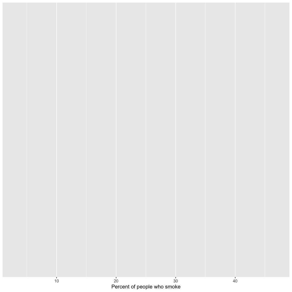
Mapping lung cancer rates to the y axis
Map our
lung_cancer_pctvalues to the y axis and give them a nice label.Solution
ggplot(data = smoking_1990) +
  aes(x = smoke_pct) +
  labs(x = "Percent of people who smoke") +
  aes(y = lung_cancer_pct) +
  labs(y = "Percent of people with lung cancer")
Excellent. We’ve now told our plot object where the x and y values are coming
from and what they stand for. But we haven’t told our object how we want it to
draw the data. There are many different plot types (bar charts, scatter plots,
histograms, etc). We tell our plot object what to draw by adding a geometry
(“geom” for short) to our object. We will talk about many different geometries
today, but for our first plot, let’s draw our data using the “points” geometry
for each value in the data set. To do this, we add geom_point() to our plot
object:
ggplot(data = smoking_1990) +
  aes(x = smoke_pct) +
  labs(x = "Percent of people who smoke") +
  aes(y = lung_cancer_pct) +
  labs(y = "Percent of people with lung cancer") +
  geom_point()
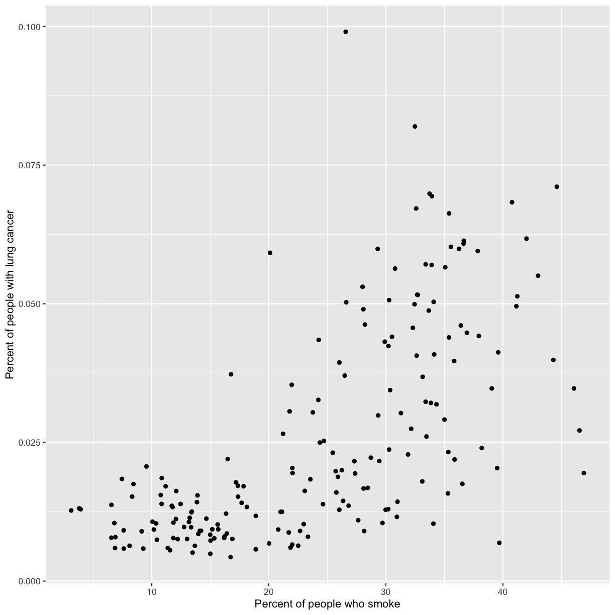
Now we’re really getting somewhere. It finally looks like a proper plot! We can now see a trend in the data. It looks like countries with greater smoking rates tend to have higher lung cancer rates, though it’s important to remember that we can’t infer causality from this plot alone.
Let’s add a title to our plot to make that clearer.
Again, we will use the labs() function, but this time we will use the title = argument.
ggplot(data = smoking_1990) +
aes(x = smoke_pct) +
labs(x = "Percent of people who smoke") +
aes(y = lung_cancer_pct) +
labs(y = "Percent of people with lung cancer") +
geom_point() +
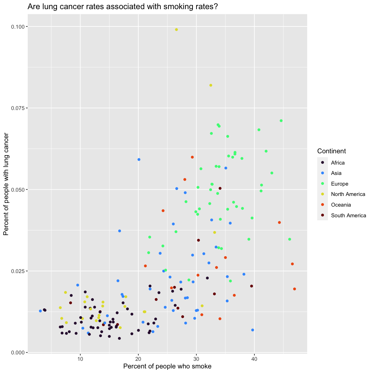
labs(title = "Are lung cancer rates associated with smoking rates?")
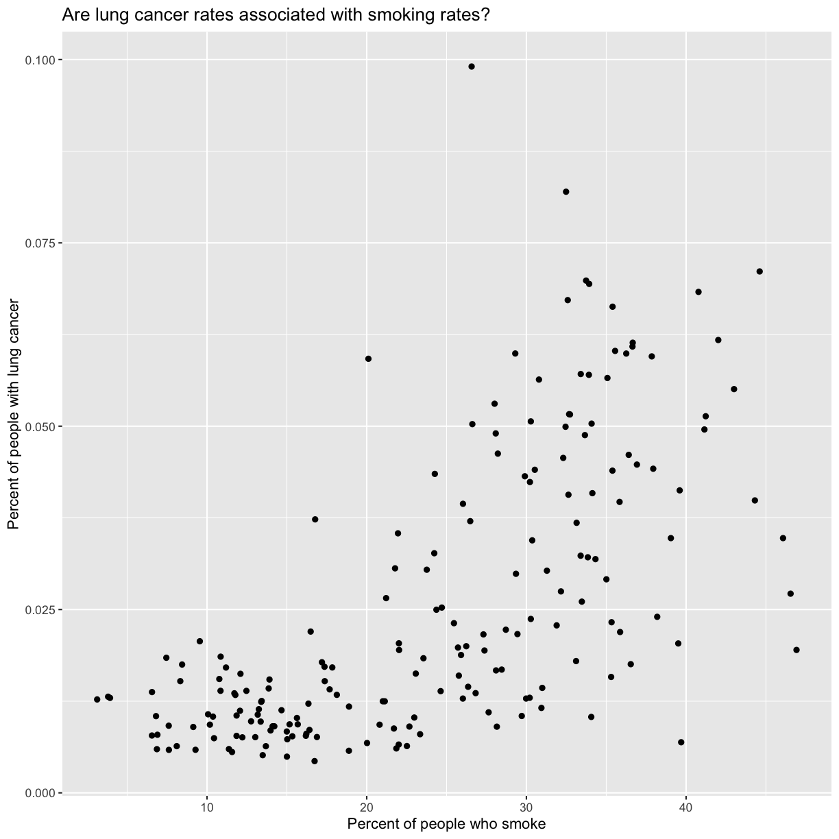
No one can deny we’ve made a very handsome plot!
We can immediately see that there is a positive association between lung cancer rates and smoking rates.
But now looking at the data, we might be curious about learning more about the points that are the extremes of
the data. We know that we have two more pieces of data in the smoking_1990
object that we haven’t used yet. Maybe we are curious if the different
continents show different patterns in smoking rates and lung cancer rates. One thing we
could do is use a different color for each of the continents. To map the
continent of each point to a color, we will again use the aes() function.
Color the points by continent
To color the points by continent, you will need to add that to your aesthetic function. Fill in the blank below with the correct column from your data to make this happen.
ggplot(data = smoking_1990) +
  aes(x = smoke_pct) +
  labs(x = "Percent of people who smoke") +
  aes(y = lung_cancer_pct) +
  labs(y = "Percent of people with lung cancer") +
  geom_point() +
  labs(title = "Are lung cancer rates associated with smoking rates?") +
  aes(_____)
What information can you learn from the plot?
Solution
ggplot(data = smoking_1990) +
  aes(x = smoke_pct) +
  labs(x = "Percent of people who smoke") +
  aes(y = lung_cancer_pct) +
  labs(y = "Percent of people with lung cancer") +
  geom_point() +
  labs(title = "Are lung cancer rates associated with smoking rates?") +
 aes(color = continent)
Here we can see that in 1990 the African countries tended to have much lower smoking and lung cancer rates than many other continents.
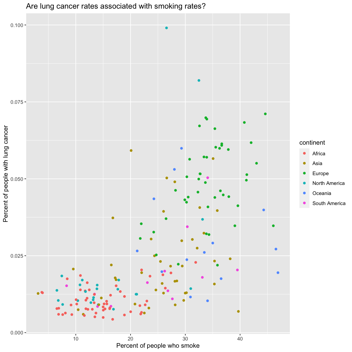
Notice that when we add a mapping for
color, ggplot automatically provided a legend for us. It took care of assigning
different colors to each of our unique values of the continent variable. (Note
that when we mapped the x and y values, those drew the actual axis labels, so in
a way the axes are like the legends for the x and y values).
The colors that ggplot uses are determined by the color “scale”. Each aesthetic value we can supply (x, y, color, etc) has a corresponding scale. Let’s change the colors to make them a bit prettier. While we’re at it, let’s capitalize the legend title too.
ggplot(data = smoking_1990) +
  aes(x = smoke_pct) +
  labs(x = "Percent of people who smoke") +
  aes(y = lung_cancer_pct) +
  labs(y = "Percent of people with lung cancer") +
  geom_point() +
  labs(title = "Are lung cancer rates associated with smoking rates?") +
  aes(color = continent) +
  scale_color_brewer(palette = "Set2") +
  labs(color = "Continent")
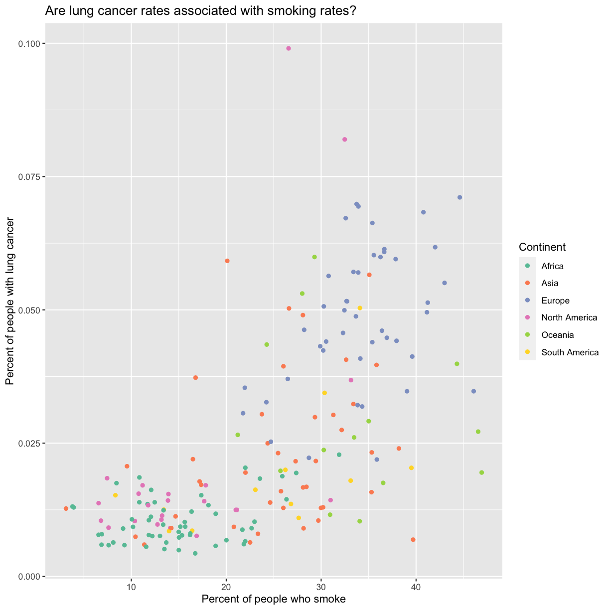
The scale_color_brewer() function is just one of many you can use to change
colors. There are bunch of “palettes” that are build in. You can view them all
by running RColorBrewer::display.brewer.all() or check out the Color Brewer
website for more info about choosing plot colors.
Check out the bonus exercise below for even more options.
Bonus Exercise: Changing colors
There are lots of ways to change colors when using ggplot. The
scale_color_brewer()function is one of many you can use to change colors. There are bunch of “palettes” that are build in. You can view them all by runningRColorBrewer::display.brewer.all()or check out the Color Brewer website for more info about choosing plot colors. There are also lots of other fun options:Play around with different color palettes. Feel free to install another package and choose one of those if you want. Pick your favorite!
Solution
You can use RColorBrewer::display.brewer.all() to pick a color palette. As a bonus, you can also use one of the packages listed above. Here’s an example:
ggplot(data = smoking_1990) +
  aes(x = smoke_pct) +
  labs(x = "Percent of people who smoke") +
  aes(y = lung_cancer_pct) +
  labs(y = "Percent of people with lung cancer") +
  geom_point() +
  labs(title = "Are lung cancer rates associated with smoking rates?") +
  aes(color = continent) +
  labs(color = "Continent") +
  scale_color_viridis_d(option = "turbo")
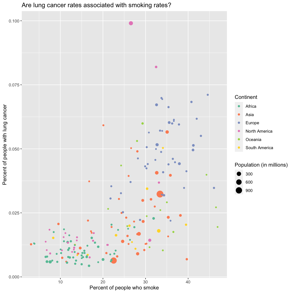
Since we have the data for the population of each country, we might be curious about the relationship between population, smoking rates, and lung cancer rates. Do you think larger countries will have a greater or lower lung cancer rate? Let’s find out by mapping the population of each country to the size of our points.
Changing point sizes
Map the population of each country to the size of our points. HINT: Is size an aesthetic or a geometry? If you’re stuck, feel free to Google it, or look at the help menu.
Solution
ggplot(data = smoking_1990) + aes(x = smoke_pct) + labs(x = “Percent of people who smoke”) + aes(y = lung_cancer_pct) + labs(y = “Percent of people with lung cancer”) + geom_point() + labs(title = “Are lung cancer rates associated with smoking rates?”) + aes(color = continent) + scale_color_brewer(palette = “Set2”) + labs(color = “Continent”) ```
There doesn’t seem to be a very strong association with population size. We also got another legend here for size, which is nice, but the values look a bit ugly in scientific notation. Let’s divide all the values by 1,000,000 and label our legend “Population (in millions)”
ggplot(data = smoking_1990) +
  aes(x = smoke_pct) +
  labs(x = "Percent of people who smoke") +
  aes(y = lung_cancer_pct) +
  labs(y = "Percent of people with lung cancer") +
  geom_point() +
  labs(title = "Are lung cancer rates associated with smoking rates?") +
  aes(color = continent) +
  scale_color_brewer(palette = "Set2") +
  labs(color = "Continent") +
  aes(size = pop/1000000) +
  labs(size = "Population (in millions)")

This works because you can treat the columns in the aesthetic mappings just like any other variables and can use functions to transform or change them at plot time rather than having to transform your data first.
Good work! Take a moment to appreciate what a cool plot you made with a few lines of code. To fully view its beauty you can click the “Zoom” button in the Plots tab - it will break free from the lower right corner and open the plot in its own window.
Bonus Exercise: Changing shapes
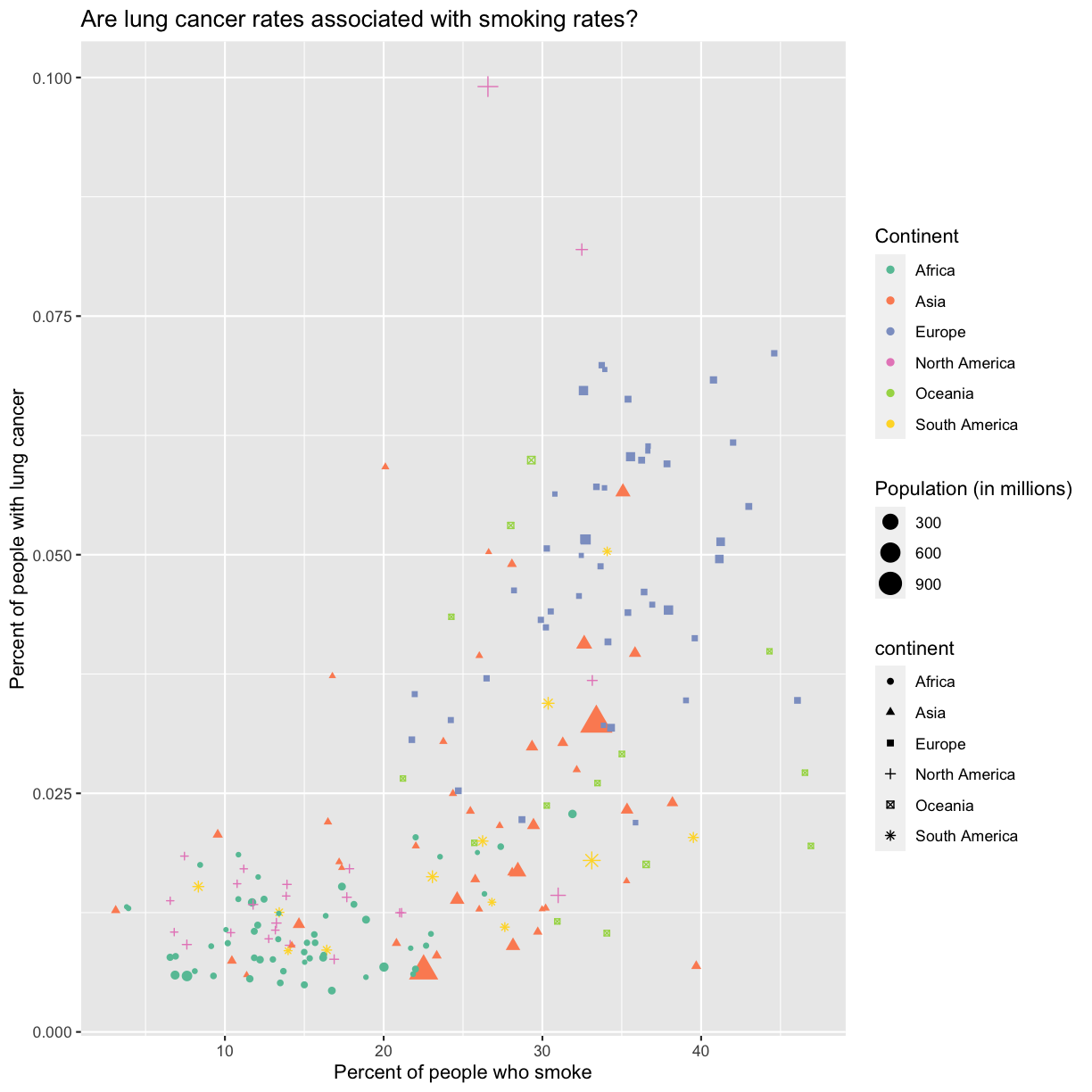
Instead of (or in addition to) color, change the shape of the points so each continent has a different shape. (I’m not saying this is a great thing to do - it’s just for practice!) HINT: Is shape an aesthetic or a geometry? If you’re stuck, feel free to Google it, or look at the help menu.
Solution
You’ll want to use the
aesaesthetic function to change the shape:ggplot(data = smoking_1990) + aes(x = smoke_pct) + labs(x = "Percent of people who smoke") + aes(y = lung_cancer_pct) + labs(y = "Percent of people with lung cancer") + geom_point() + labs(title = "Are lung cancer rates associated with smoking rates?") + aes(color = continent) + scale_color_brewer(palette = "Set2") + labs(color = "Continent") + aes(size = pop) + aes(size = pop/1000000) + labs(size = "Population (in millions)") + aes(shape = continent)
For our first plot we added each line of code one at a time so you could see the
exact affect it had on the output. But when you start to make a bunch of plots,
we can actually combine many of these steps so you don’t have to type as much.
For example, you can collect all the aes() statements and all the labs()
together. A more condensed version of the exact same plot would look like this:
ggplot(data = smoking_1990) +
  aes(x = smoke_pct, y = lung_cancer_pct, color = continent, size = pop/1000000) +
  geom_point() +
  scale_color_brewer(palette = "Set2") +
  labs(x = "Percent of people who smoke", y = "Percent of people with lung cancer",
    title = "Are lung cancer rates associated with smoking rates?", color = "Continent", size = "Population (in millions)")
Storing our plot
We learned about how to save things to object names in the previous lesson. We can do the same thing with plots! Store our final plot in an object called
cancer_v_smoke.Solution
 cancer_v_smoke <- ggplot(data = smoking_1990) +
   aes(x = smoke_pct, y = lung_cancer_pct, color = continent, size = pop/1000000) +
   geom_point() +
   scale_color_brewer(palette = "Set2") +
   labs(x = "Percent of people who smoke", y = "Percent of people with lung cancer",
     title = "Are lung cancer rates associated with smoking rates?", color = "Continent", size = "Population (in millions)")
Saving our first plot
Let’s say you want to share your plot with friends or co-workers who aren’t running R. It’s wise to keep all the code you used to draw the plot, but sometimes you need to make a PNG or PDF version of the plot so you can share it with your PI or post it to your Instagram story.
To save your plot, you can use the ggsave() function. A few things about ggsave() (the good and the bad):
- [The bad] By default,
ggsave()will save the last plot you made, but this can get confusing so it’s best to create a plot object and then save the specific plot you’re interested in instead. - [The neutral] The default width and height are sometimes not great options,
but you can supply
width=andheight=arguments to change them (the default values are in inches). - [The good] It will determine the file type based on the name you provide.
Let’s save our plot (with an informative name) as a 4x6 inch png:
ggsave(filename = "figures/cancer_v_smoke.png", plot = cancer_v_smoke, width = 6, height = 4)
Debugging code
Debugging is the process of finding and fixing errors or unexpected outputs in your code. Even well seasoned coders run into bugs all the time.
Here are some strategies of how programmers try to deal with coding errors:
- Don’t panic. Bugs are a normal part of the coding process.
- If you are getting an error message, read the error message carefully. Unfortunately, not all error messages are well written and it may not be obvious at first what is wrong.
- Check for typos.
- Check that your parentheses and quotes are balanced and check that you haven’t misspelled a variable or function name, or used the wrong one.
- It’s difficult to identify the exact location where an error starts so you may have to look at lines before the line where the error was reported.
- In RStudio, look at the code coloring to find anything that looks off. RStudio will also put a red x or an yellow exclamation point to the left of lines where there is a syntax error.
- Try running each command on its own.
- Before each command, check that you are passing the values you expect.
- After each command, verify that the results seem sensible.
- If you’re getting an error, search online for the error message along with the function that is not working.
Consider checking out the following resources to learn more about it.
- “5 Essential Tips to Debug Any Piece of Code” by mayuko [video, 8min] - Good general advice for debugging.
- “Object of type ‘closure’ is not subsettable” by Jenny Bryan [video, 50min] - A great talk with R specific advice about dealing with errors as a data scientist.
Understanding common bugs
Sometimes you accidentally type things wrong and get unexpected results or errors. We call these mis-types “bugs”. Let’s go through some common ones. The most important things to remember are:
- The order of parentheses, quotes, commas, and plusses matters.
- Sometimes you accidentally forget a plus where you need one or include one where you don’t.
For each of the examples below, figure out what the bug is and how to fix it. Feel free to copy/paste into RStudio to help you figure it out.
# Bug 1

 ggplot(data = smoking_1990) +
 aes(x = "smoke_pct", y = lung_cancer_pct, color = continent, size = pop/1000000) +
   geom_point() +
   labs(x = "Percent of people who smoke", y = "Percent of people with lung cancer",
        title = "Are lung cancer rates associated with smoking rates?",
       color = "Continent", size = "Population (in millions)")

# Bug 2

ggplot(data = smoking_1990) +
   aes(x = smoke_pct, y = lung_cancer_pct, color = continent, size = pop/1000000) +
   geom_point() +
   labs(x = "Percent of people who smoke", y = "Percent of people with lung cancer",
        title = "Are lung cancer rates associated with smoking rates?",
       color = "Continent", size = "Population (in millions)"))

# Bug 3
ggplot(data = smoking_1990) +
   aes(x = smoke_pct, y = lung_cancer_pct, color = continent, size = pop/1000000) +
   geom_point() +
   labs(x = "Percent of people who smoke", y = "Percent of people with lung cancer",
        title = "Are lung cancer rates associated with smoking rates?",
       color = "Continent" size = "Population (in millions)")
Solution
Bug 1: We generated a plot, but it doesn’t look like what we expect. The bug is in our mapping of aesthetics:
geom_point(aes(x = "smoke_pct", y = lung_cancer_pct, color = continent, size = pop/1000000)). Because"smoke_pct"is in quotation marks, ggplot understands that as a single value, rather than an aesthetic mapped to thesmoke_pctvariable in thesmoking_1990dataset. To correct this bug, remove the quotes from"smoke_pct"so that ggplot looks for thesmoke_pctcolumn in our dataset.Bug 2: This code generates the following error:
Error: unexpected ')' in:
"      scale_color_brewer(palette = "Set2") +
     labs(x = "Percent of people who smoke", y = "Percent of people  with lung cancer", title = "Are lung cancer rates associated with smoking rates?", size = "Population (in millions)"))"
Although it might be alarming to get this error, it’s actually quite helpful! You can see that the error points out that we have an unexpected closed parentheses “)” in the last two lines of our code. Look closely, and you’ll see that we accidentally put an extra “)” on the
labs()layer in the last line of code.Bug 3: This code generates the following error:
Error: unexpected symbol in:
"                       title = "Are lung cancer rates associated with smoking rates?",
                      color = "Continent" size"
This error message tells us that there was something unexpected in the
labs()funtion on either the line where we specified the title or the color. These errors can be some of the hardest to figure out, because the message is not very specific. However, if you look closely, yu will see that we are missing a comma betweencolor = "Continent"andsize = "Population (in millions)"inside the label function.
Recap of what we’ve learned so far
Now that we’ve made our first plot, let’s review the most important things to remember when plotting with ggplot. Making plots using ggplot is all about layering on information.
- First, you have to give the
ggplot()function your data.- It looks in this data for the information in the columns you tell it to use for your plot.
- Then, you have to tell ggplot what specific information from your data you want to plot and how you want that data to show up.
- You use the
aes()function for this. - Inside this function you tell it how you want the data to show up (on the x axis, on the y axis, as a color, etc.) and where that data is coming from (the column name in your datset).
- You use the
- Finally, you have to tell ggplot what type of plot you want to make.
- All ggplot plot types start with the word
geom(e.g.geom_point()).
- All ggplot plot types start with the word
- You can customize the labels and colors on your plot to make them nicer and more informative.
- There’s a lot more you can customize as well. We will go into some of this later on in the lesson.
This is a lot to remember!
Pro-tip
Those of us that use R on a daily basis use cheat sheets to help us remember how to use various R functions. You can find the cheat sheets in RStudio by going to the “Help” menu and selecting “Cheat Sheets”. The ones that will be most helpful in this workshop are “Data visualization with ggplot2”, “Data Transformation with dplyr”, “R Markdown Cheat Sheet”, and “R Markdown Reference Guide”.
For things that aren’t on the cheat sheets, Google is your best friend. Even expert coders use Google when they’re stuck or trying something new!
Let’s take a moment to orient ourselves to our “Data visualization with ggplot2” cheat sheet. What we just went over is summarized in the “Basics” section in the upper left hand side of the front page of your cheat sheet. The other sections contain more information about different geometries and aesthetics you can use in your plots. We will go over some of these in the next section.
Bonus Exercise: Make your own scatter plot
Now create your own scatter plot comparing population and percent of people who smoke. Looking at your plot, can you guess which two countries have the largest populations?
If you have extra time, customize your plot however you want. If there’s something you want to do but don’t know how, try searching on the internet for it.
Solution
ggplot(data = smoking_1990) +
  aes(x = pop, y = smoke_pct) +
  geom_point()
(China and India are the two countries with large populations.)
Plotting for data exploration
Now that we’ve made our first plot, we’re going to dig into other ways to visualize data using ggplot. The main goal here is to find meaningful patterns in complex data and create visualizations to convey those patterns.
Discrete Plots
The plot type we used to make our first plot, geom_point, works when both the x and y values are continuous. But sometimes one of your values may be discrete (i.e. categorical).
We’ve previously used the discrete values of the continent column to color in our points and lines. But now let’s try moving that variable to the x axis. Let’s say we are curious about comparing the distribution of the lung cancer rates for each of the different continents for the smoking_1990 data. We can do so using a box plot. Try this out yourself in the exercise below!
Plotting and interpreting box plots
Using the
smoking_1990data, use ggplot to create a box plot with continent on the x axis and lung cancer rates on the y axis. The geom you will want to use isgeom_boxplot(). You can use the examples from earlier in the lesson as a template to remember how to pass ggplot data and map aesthetics and geometries onto the plot. If you’re really stuck, feel free to use the internet as well!Which continent tends to have countries with the highest lung cancer rates? The lowest?
Solution
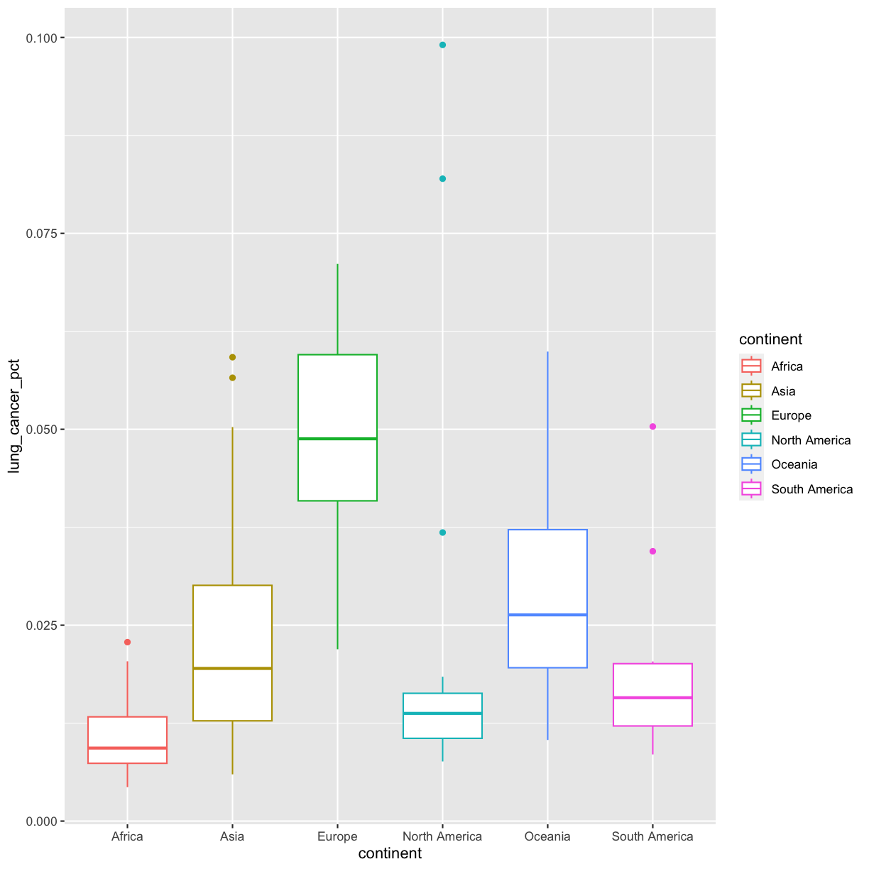
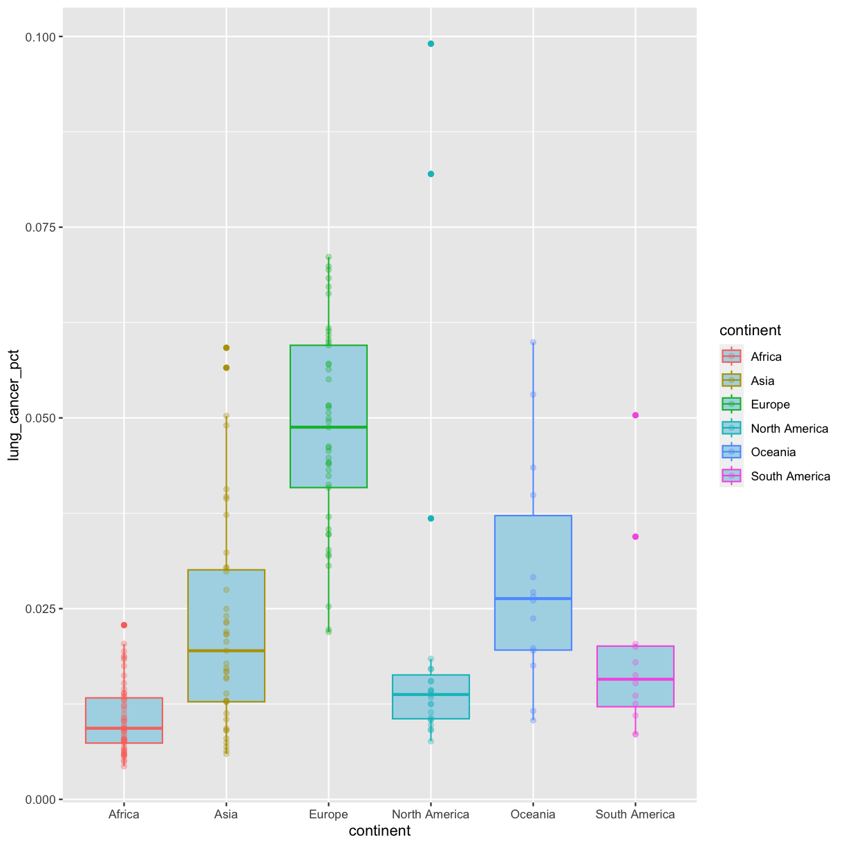
ggplot(data = smoking_1990) +
 aes(x = continent, y = lung_cancer_pct) +
 geom_boxplot()
This type of visualization makes it easy to compare the range and spread of values across groups. The “middle” 50% of the data is located inside the box and outliers that are far away from the central mass of the data are drawn as points. The bar in the middle of the box is the median. Here, we can see that the median bar for Europe is highest, indicating that countries in Europe tend to have higher rates of lung cancer than countries on other continents. Countries in Africa tend to have lower lung cancer rates than countries on other continents.
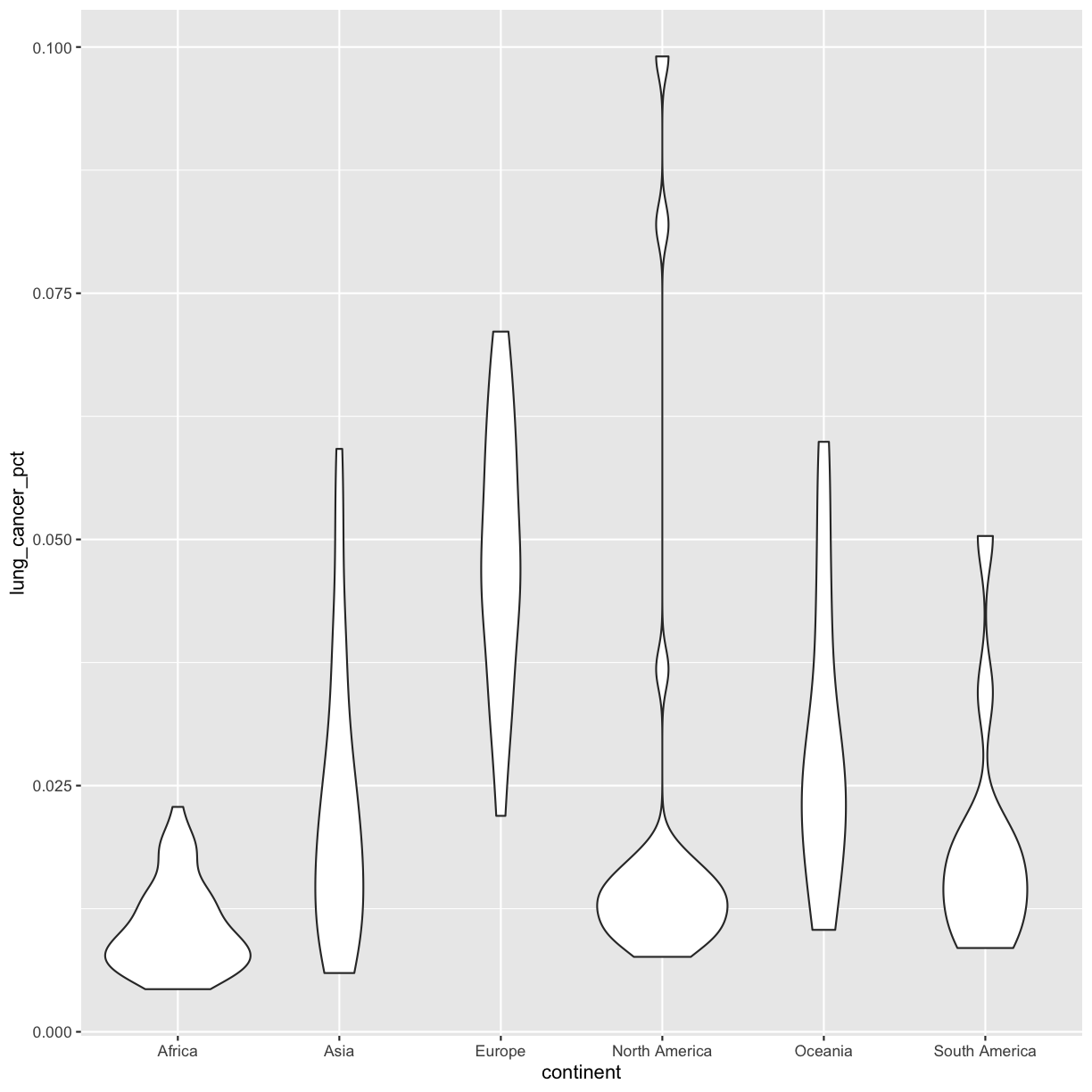
Bonus Exercise: Other discrete geoms
Take a look a the ggplot cheat sheet. Find all the geoms listed under “one discrete, one continuous.” Try replacing
geom_boxplotwith one of these other functions.Example solution
ggplot(data = smoking_1990) +
  aes(x = continent, y = lung_cancer_pct) +
  geom_violin()
Color vs. Fill
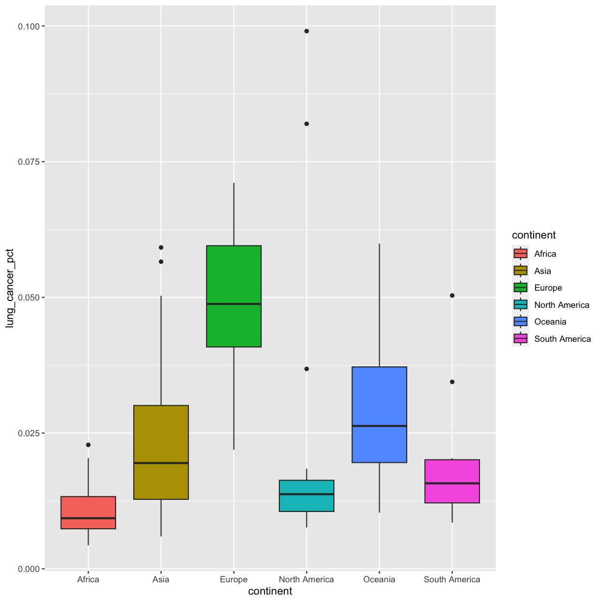
Let’s take the boxplot that we made previously and add code to make the color corresponds to continent. Remember how to do that?
ggplot(data = smoking_1990) +
  aes(x = continent, y = lung_cancer_pct, color = continent) +
  geom_boxplot()
Well, that didn’t get all that colorful. That’s because objects like these boxplots have two different parts that have a color: the shape outline, and the inner part of the shape. For geoms that have an inner part, you change the fill color with fill= rather than color=, so let’s try that instead:
ggplot(data = smoking_1990) +
  aes(x = continent, y = lung_cancer_pct, fill = continent) +
  geom_boxplot()
That got more colorful. Neither one of these (color vs. fill) is better than the other here, it’s more up to your personal preference.
Let’s say we want to change the fill of our plots, but to all the same color. Maybe we want our boxplots to be “lightblue”.
Quotes or no quotes?
To change the color of our boxplots to lightblue, do you think we need to put lightblue in quotes or not? Why?
Solution
We want to put it in quotes because it isn’t a column name in our dataset or a variable in our environment.
Let’s try it out without quotes first:
ggplot(data = smoking_1990) +
  aes(x = continent, y = lung_cancer_pct, fill = lightblue) +
  geom_boxplot()
Error in `geom_boxplot()`:
! Problem while computing aesthetics.
ℹ Error occurred in the 1st layer.
Caused by error:
! object 'lightblue' not found
Like we just discussed, we get an error because when we don’t include quotes, R looks for the lightblue object in our dataframe and our environment, but it doesn’t find it there. Instead, we have to put it in quotes so that R knows not to search for that variable, but instead to actually use the word itself:
ggplot(data = smoking_1990) +
  aes(x = continent, y = lung_cancer_pct, fill = "lightblue") +
  geom_boxplot()
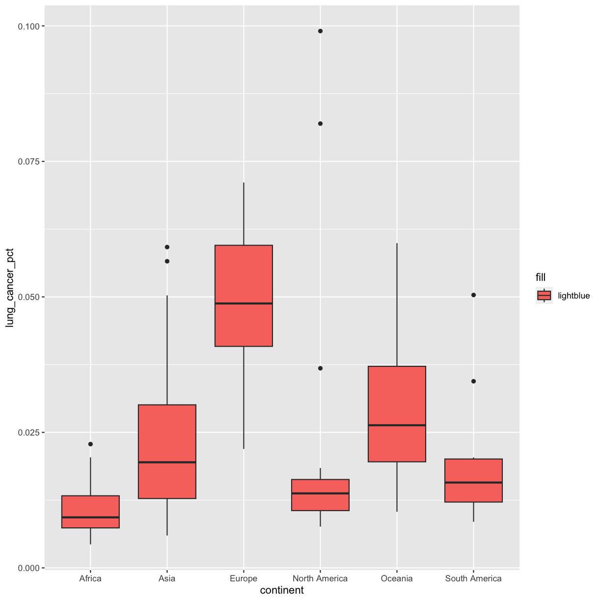
Hmm that’s still not quite what we want. In this example, we placed the fill inside the aes() function, which maps aesthetics to data. In this case, we only have one value: the word “lightblue”. Instead, let’s do this by explicitly setting the color aesthetic inside the geom_boxplot() function. Because we are assigning a color directly and not using any values from our data to do so, we do not need to use the aes() mapping function. Let’s try it out:
ggplot(data = smoking_1990) +
  aes(x = continent, y = lung_cancer_pct) +
  geom_boxplot(fill = "lightblue")

That’s better! R knows many color names. You can see the full list if you run colors() in the console. Since there are so many, you can randomly choose 10 if you run sample(colors(), size = 10).
Choosing a color
Use
sample(colors(), size = 10)a few times until you get an interesting sounding color name and swap that out for “lightblue” in the box plot example.
Layers
So far we’ve only been adding one geom to each plot, but each plot object can actually contain multiple layers and each layer has it’s own geom. Now let’s add a layer of points on top of our boxplot that will show us the “raw” data:
ggplot(data = smoking_1990) +
  aes(x = continent, y = lung_cancer_pct) +
  geom_boxplot(fill = "lightblue") +
  geom_point()

We’ve drawn the points but most of them stack up on top of each other. One way to make it easier to see all the data is to change the transparency of the points. We can do this using the alpha argument, which decides how transparent to make the points. It takes a value between 0 and 1 where 0 is entirely transparent and 1 is entirely opaque (the default).
Inside
aes()orgeom?Let’s say we want to change the transparency of our points to an alpha of 0.3. Do we want alpha to go inside our
aes()function or ourgeom_boxplot()? Why? Test out both and see if you’re right!Solution
We want alpha to go inside
geom_boxplot()since we’re telling ggplot the number we want it to use; it’s not coming from our data.ggplot(data = smoking_1990) + aes(x = continent, y = lung_cancer_pct) + geom_boxplot(fill = "lightblue") + geom_point(alpha = 0.3)
Bonus: Too many overlapping points for alpha to work?
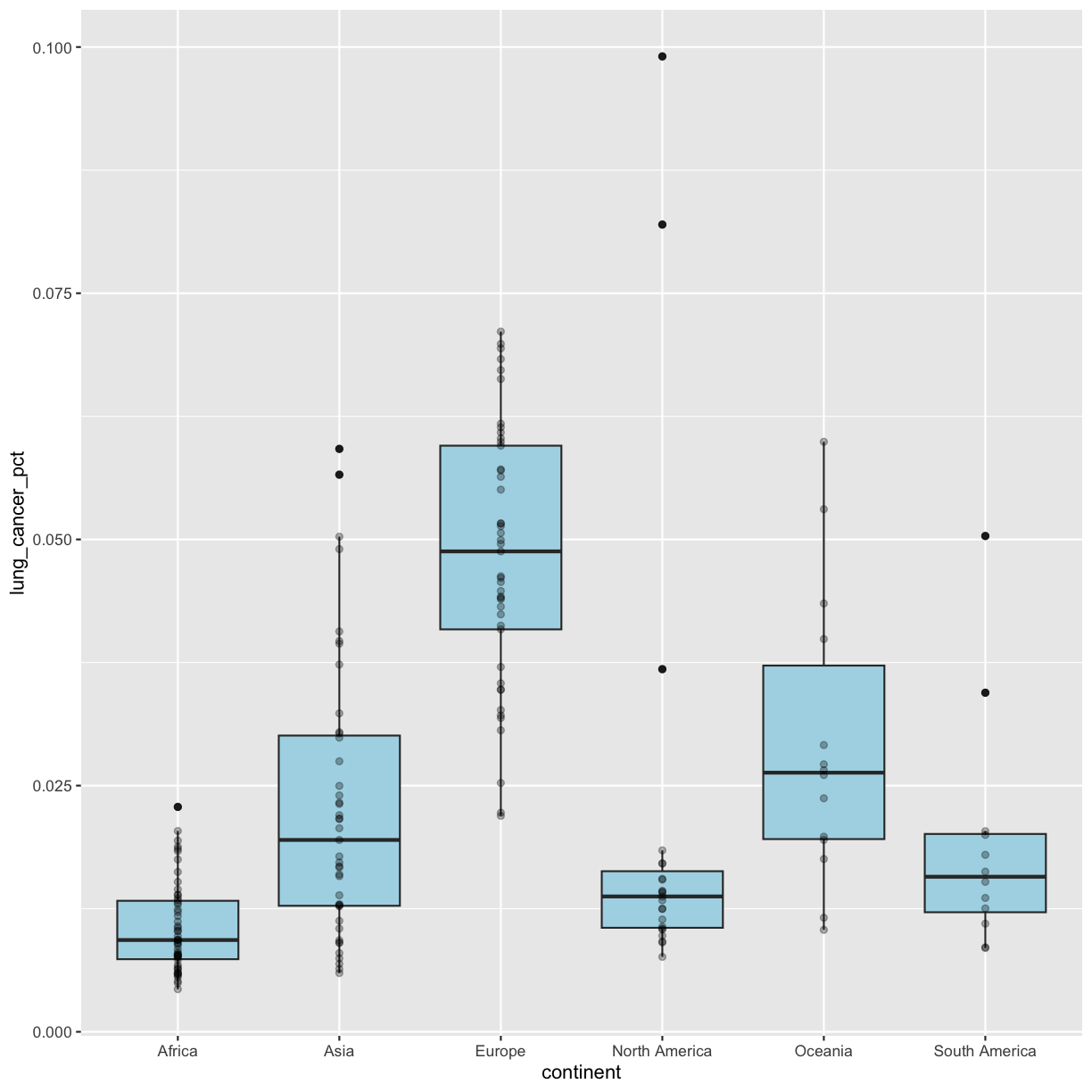
We have many observations/data points, so even making the points transparent doesn’t really help us see them! Another option is to “jitter” the points. This adds some random variation to the position of the points so you can see them better. We can do this using
geom_jitter().WARNING!!!
geom_jitter()changes the position of points and should therefore only be used for discrete variables that don’t have numerical values!!!Since we are plotting a discrete value on the x axis, and a continuous value on the y axis, we will need to tell
geom_jitter()not to change the y value positions. We can do this by settingheight = 0inside the geom. We will also modify the degree to which points are jittered on the x axis by setting thewidthargument. Feel free to play around withwidthto get a plot that you like. Remember, we can only do this because the x axis is discrete!ggplot(data = smoking_1990) + aes(x = continent, y = lung_cancer_pct) + geom_boxplot(fill = "lightblue") + geom_jitter(alpha = 0.3, height = 0, width = 0.05)
That looks better!
Predicting output
What do you think will happen if you switch the order of
geom_boxplot()andgeom_point()? Why? Test it out to see if you were right.Solution
Since we plot the
geom_point()layer first, the boxplot layer is placed on top of thegeom_point()layer, so we cannot see a lot of the points.ggplot(data = smoking_1990) + aes(x = continent, y = lung_cancer_pct) + geom_point(, alpha = 0.3) + geom_boxplot(fill = "lightblue")

Going back to having the points on top, let’s color the points by continent. If we add a color aesthetic to the plot, then both the boxplot and the points are colored by continent:
ggplot(data = smoking_1990) +
  aes(x = continent, y = lung_cancer_pct, color = continent) +
  geom_boxplot(fill = "lightblue") +
  geom_point(alpha = 0.3)
So how do we make it so that just the points are colored but not the boxplots? Each layer can have it’s own set of aesthetic mappings. So far we’ve been using aes() outside of the other functions. When we do this, we are setting the “default” aesthetic mappings for the plot. But we can also set the asethetics inside the specific geom that we want to change. To do that, you can place an additional aes() inside of that layer:
ggplot(data = smoking_1990) +
  aes(x = continent, y = lung_cancer_pct) +
  geom_boxplot(fill = "lightblue") +
  geom_point(aes(color = continent), alpha = 0.3)
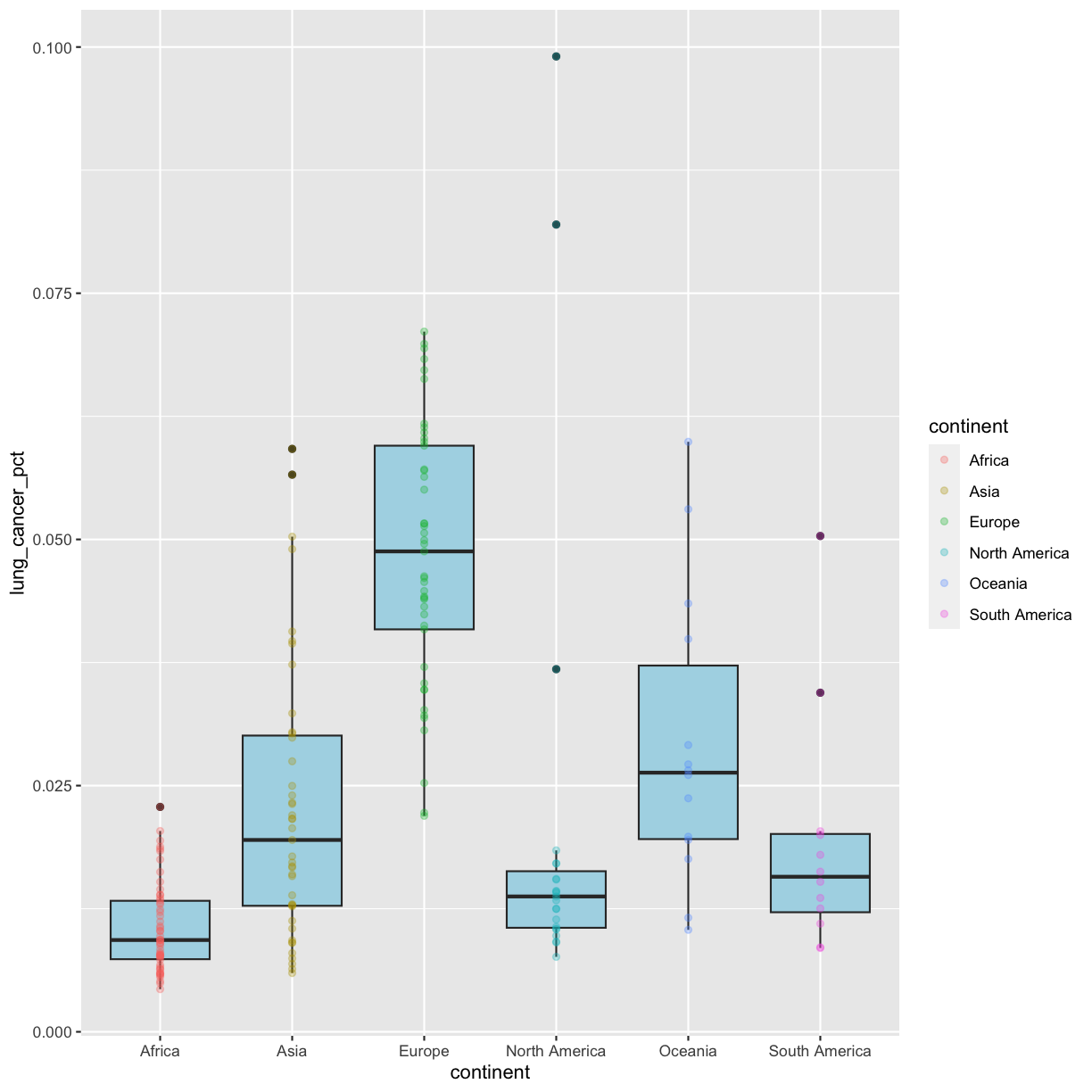
Nice! Both geom_boxplot() and geom_point() will inherit the default values of aes(continent, lung_cancer_pct) in the base plot, but only geom_jitter will also use aes(color = continent).
Bonus: Aesthetics inside the
ggplot()functionInstead of mapping our aesthetics to each geom, we can provide default aesthetics by passing the values to the
ggplot()function call. Any aesthetics we want to be specific to a layer, we would keep in the geom function for that layer:ggplot(data = smoking_1990, mapping = aes(x = continent, y = lung_cancer_pct)) + geom_boxplot(fill = "lightblue") + geom_point(aes(color = continent), alpha = 0.3)
Here, both
geom_boxplot()andgeom_point()will inherit the default values ofaes(continent, lung_cancer_pct)in the base plot, but onlygeom_point()will also useaes(color = continent).
Bonus Exercise: Make your own violin plot
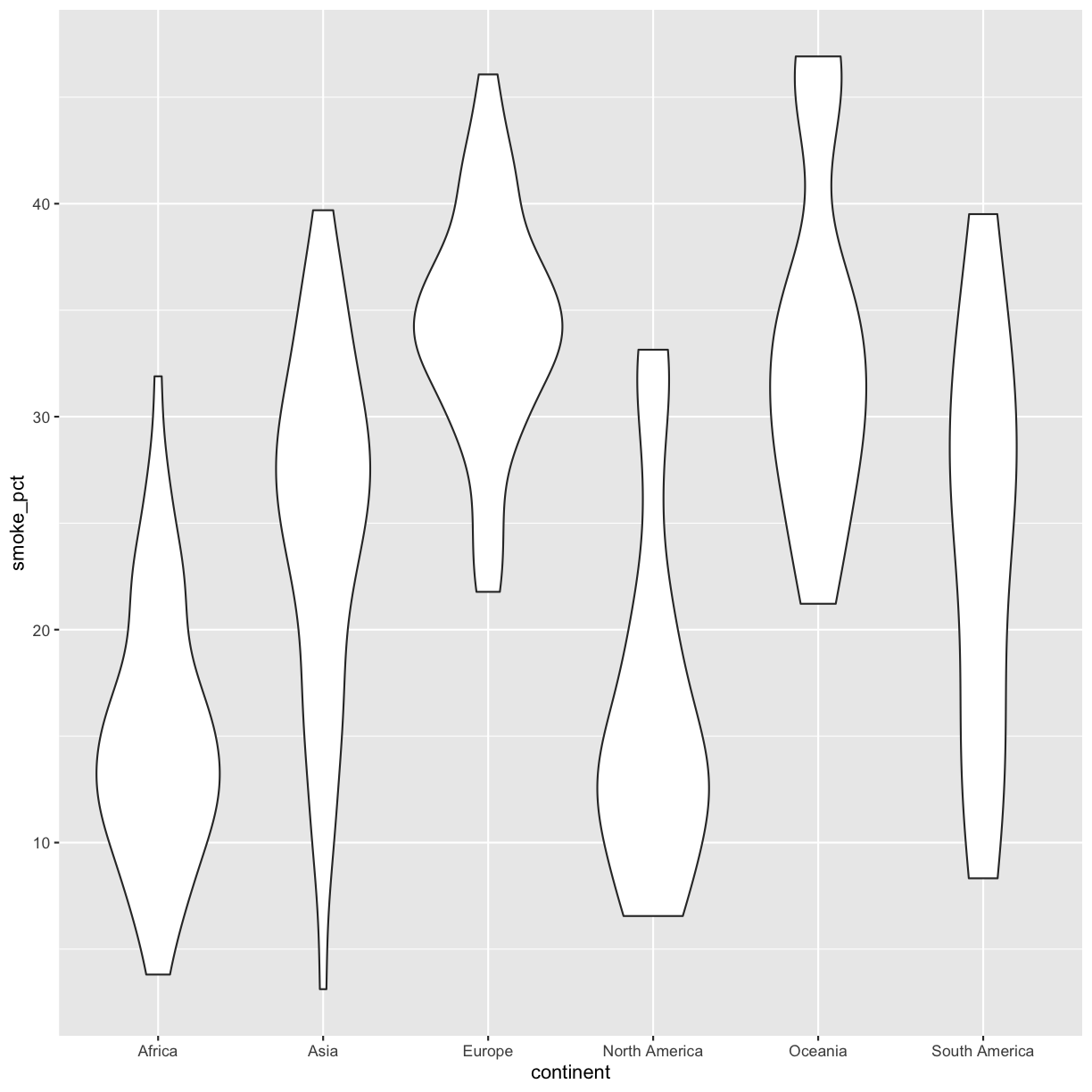
Now create a violin plot comparing percent of people in a country who smoke by continent.
If you have extra time, customize your plot however you want. If there’s something you want to do but don’t know how, try searching on the internet for it.
Solution
ggplot(data = smoking_1990) +
  aes(x = continent, y = smoke_pct) +
  geom_violin()
Univariate Plots
We jumped right into make plots with multiple columns. But what if we wanted to take a look at just one column? This can be really useful if we want to understand how certain continuous exposures or outcomes are distributed in our dataset. In that case, we only need to specify a mapping for x and choose an appropriate geom.
Univariate continuous
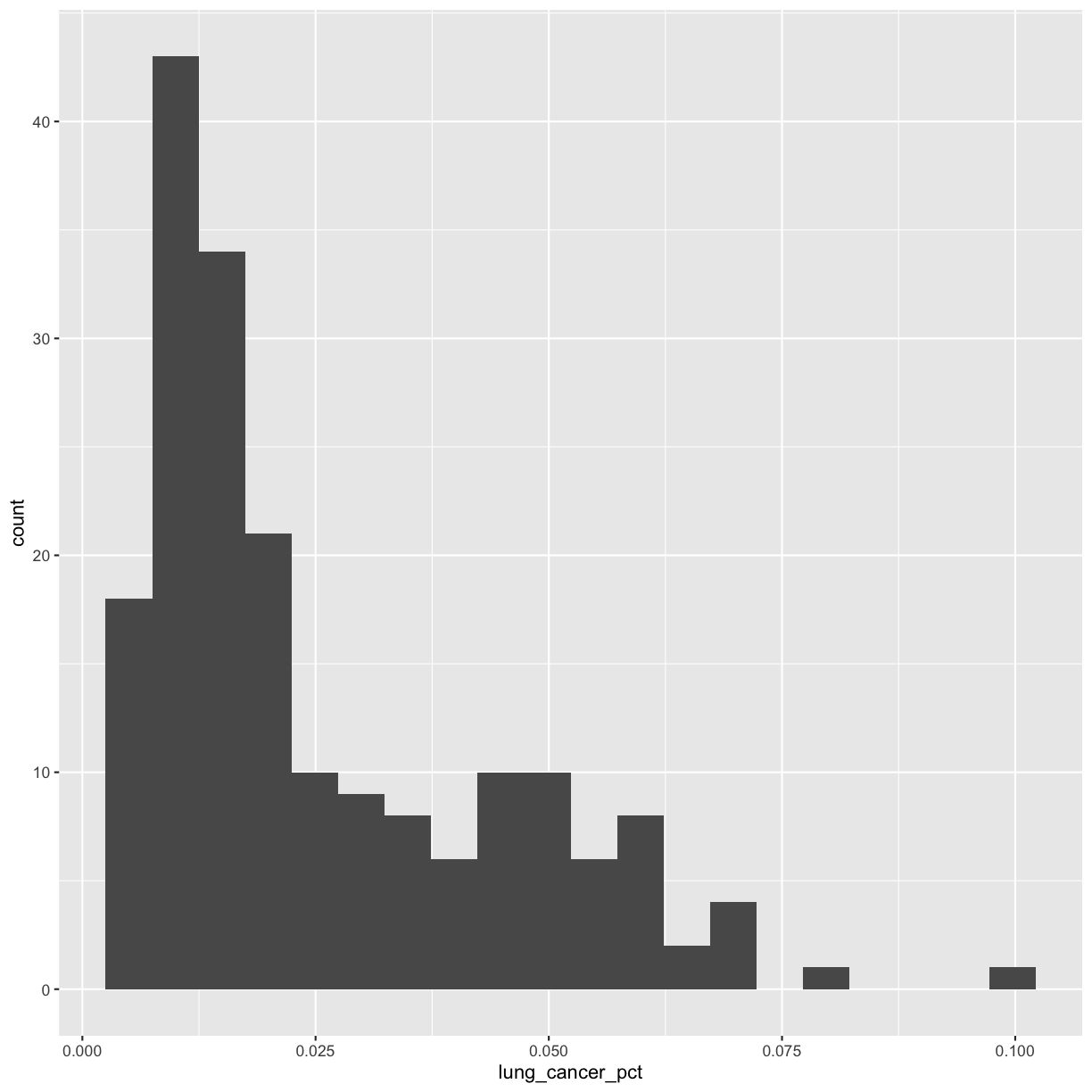
Let’s start with a histogram to see the range and spread of the lung cancer rates:
ggplot(smoking_1990) +
  aes(x = lung_cancer_pct) +
  geom_histogram()
`stat_bin()` using `bins = 30`. Pick better value with `binwidth`.
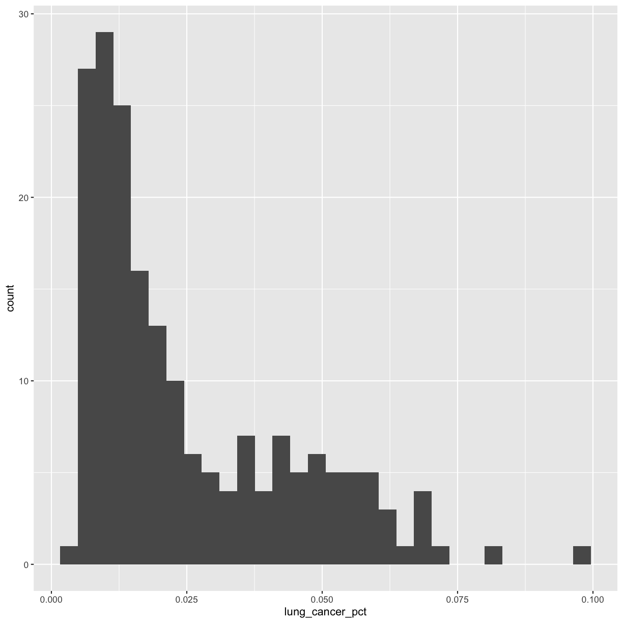
This plot shows us that many of the lung cancer rates in our dataset are really low (less than 0.025%), but there are some outliers with higher rates. Another word for data with this shape is right-skewed, because it has a long tail on the right side of the histogram.
When you ran the code to make the histogram, you should not only see the plot in the plot window, but also a message telling you to choose a better bin value. Histograms can look very different depending on the number of bars you decide to draw. The default is 30. Let’s try setting a different value by explicitly passing a bin= argument to the geom_histogram later.
ggplot(smoking_1990) +
  aes(x = lung_cancer_pct) +
  geom_histogram(bins=20)

Try different values like 5 or 50 to see how the plot changes.
Bonus Exercise: One variable plots
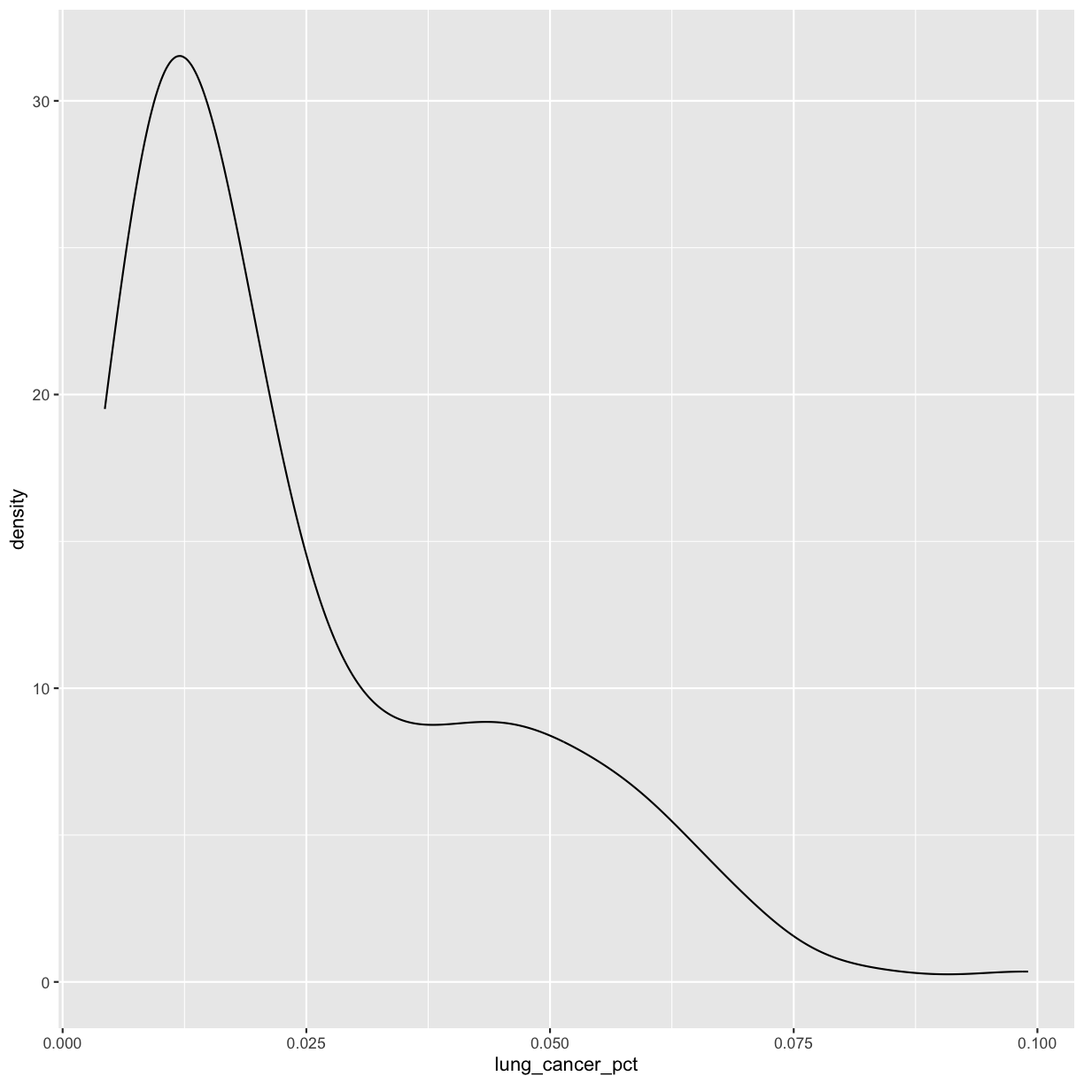
Rather than a histogram, choose one of the other geometries listed under “One Variable” continuous plots on the ggplot cheat sheet.
Example solution
ggplot(smoking_1990) +
  aes(x = lung_cancer_pct) +
  geom_density()
Univariate discrete
What if we want to plot a univariate discrete variable, like continent? For this, we can use a bar chart.
Exercise: Discrete univariate plots
Create a bar plot of
continentthat shows the number of data points we have for each continent. You can try guessing the geom or look it up on the cheat sheet or Internet. Which continents have the most and fewest countries? How can you tell?Example solution
ggplot(smoking_1990) +
  aes(x = continent) +
  geom_bar()
Africa has the most countries and Oceania has the fewest. We can tell this because Africa has the highest bar and Oceania has the lowest.
Facets
If you have a lot of different columns to try to plot or have distinguishable subgroups in your data, a powerful plotting technique called faceting might come in handy. When you facet your plot, you basically make a bunch of smaller plots and combine them together into a single image. Luckily, ggplot makes this very easy. Let’s start with the histogram that we were just working with:
ggplot(smoking_1990) +
  aes(x = lung_cancer_pct) +
  geom_histogram(bins=20)
Now, let’s draw a separate box for each continent. We can do this with facet_wrap()
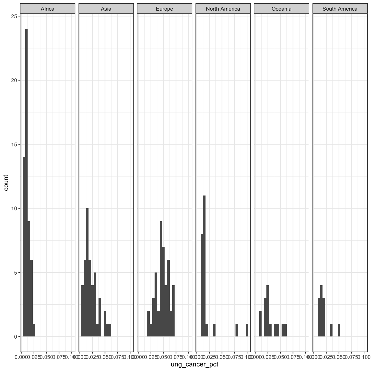
ggplot(smoking_1990) +
  aes(x = lung_cancer_pct) +
  geom_histogram(bins=20) +
  facet_wrap(vars(continent))
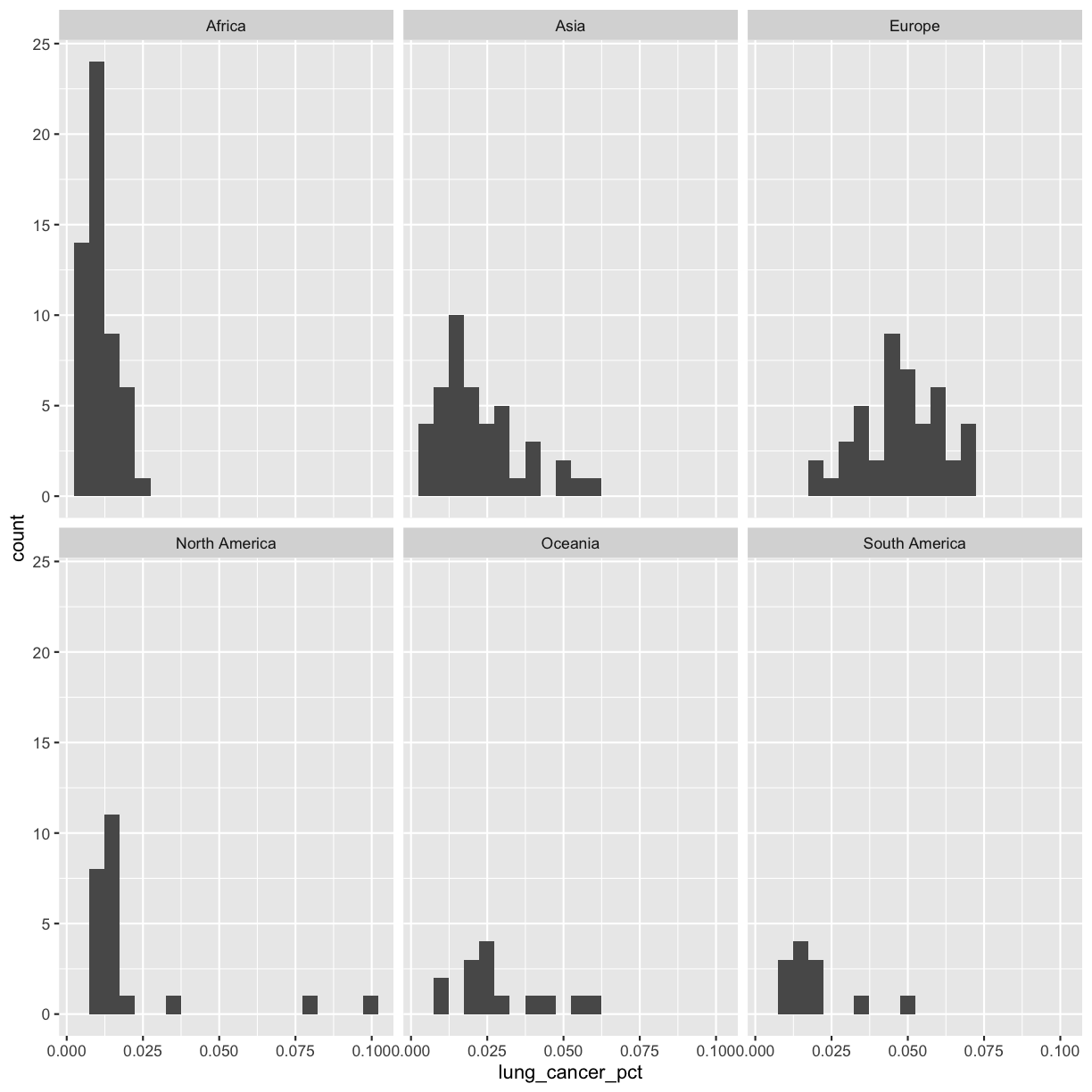 Now, it’s easier to see the patterns within and between continents.
Note that facet_wrap requires an extra helper function called vars() in order to pass in the column names. It’s a lot like the aes() function, but it doesn’t require an aesthetic name. We can see in this output that we get a separate box with a label for each continent so that only the values for that continent are in that box.
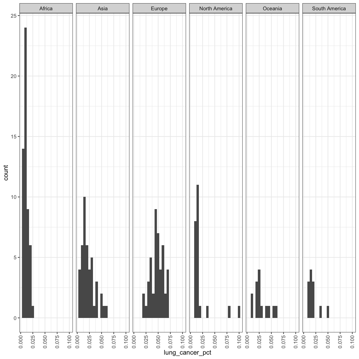
The other faceting function ggplot provides is facet_grid(). The main difference is that facet_grid() will make sure all of your smaller boxes share a common axis. In this example, we will put the boxes into columns side-by-side so that their y axes all line up. We can do this using the cols argument inside facet_grid.
ggplot(smoking_1990) +
  aes(x = lung_cancer_pct) +
  geom_histogram(bins=20) +
  facet_grid(cols = vars(continent))
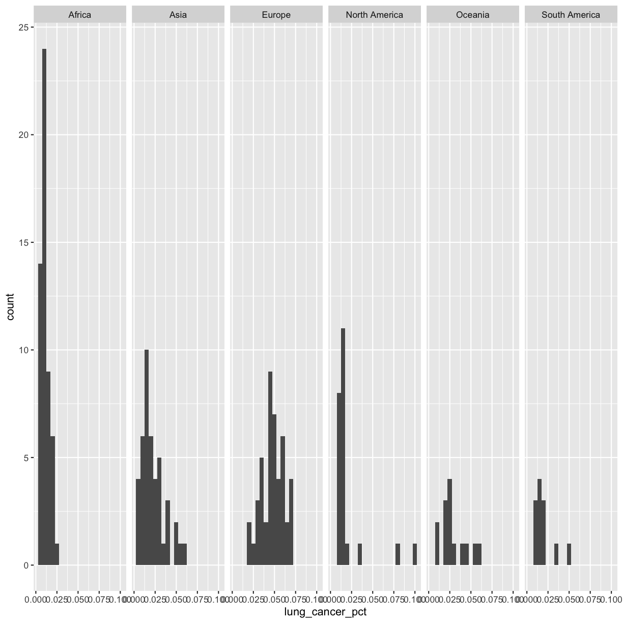
Unlike the facet_wrap output where each box got its own x and y axis, with facet_grid(), there is only one y axis along the left.
Exercise: Faceting
Facet the scatter plot we made as our first plot by continent. Are there differences in correlation between continents?
Solution
You can copy all the code from the first plot, or you can use the saved variable that we made above and add to that:
cancer_v_smoke +
  facet_wrap(vars(continent))
There don’t seem to be many differences between continents.
Bonus Exercise: Practice saving
Store the plot you made above in an object named
my_plot, and save the plot usingggsave().Example solution
my_plot <- cancer_v_smoke +
  facet_wrap(vars(continent))

ggsave("cancer_v_smoke_faceted.jpg", plot = my_plot, width=6, height=4)
Plot Themes
Our plots are looking pretty nice, but what’s with that grey background? While you can change various elements of a ggplot object manually (background color, grid lines, etc.) the ggplot package also has a bunch of nice built-in themes to change the look of your graph. For example, let’s try adding theme_bw() to our histogram:
ggplot(smoking_1990) +
  aes(x = lung_cancer_pct) +
  geom_histogram(bins=20) +
  facet_grid(cols = vars(continent)) +
  theme_bw()
Try out a few other themes, to see which you like: theme_classic(), theme_linedraw(), theme_minimal().
Rotating x axis labels
Often, you’ll want to change something about the theme that you don’t know how to do off the top of your head. When this happens, you can do an Internet search to help find what you’re looking for. To practice this, search the Internet to figure out how to rotate the x axis labels 90 degrees. Then try it out using the histogram plot we made above.
Solution
ggplot(smoking_1990) +
 aes(x = lung_cancer_pct) +
 geom_histogram(bins=20) +
 facet_grid(cols = vars(continent)) +
 theme_bw() +
  theme(axis.text.x = element_text(angle = 90, vjust = 0.5, hjust=1))
Plotting for data exploration recap
We learned a lot in this lesson! Let’s go over the key points:
- ggplot is a powerful way to make plots.
- ggplot is all about layering - you can layer different geometries, aesthetics, labels, and other information onto your plots.
- You can customize the color, size, shape, and theme of your plots.
- ggplot allows you to easily save publication-quality plots.
- There are lots of different plot types. Some of the most useful ones are:
- Scatter plots (for two continuous variables).
- Boxplots (for one discrete and one continuous variable).
- Histograms (for one continuous variable).
- Bar plots (for one discrete variable).
- Faceting allows you to easily make the same plot separated by a discrete variable of interest.
With the skills you’ve learned here, you’re now ready to start doing your own data exploration!
Applying it to your own data
Now that we’ve learned how impactful effective data visualization can be, and how to create informative visuals in R, it’s time for you to start thinking about what you want to do with your own data!
Discuss with your group your data and what type of exploratory data analysis you would like to perform.
Questions to answer:
- In 1-2 sentences, describe the information covered in your dataset.
- How large is your dataset? How many rows? How many columns?
- Write down 3 specific questions you could answer with your data set.
- Think through 3 data visualizations that can answer the questions you have. Specifically, for each one: a) Write down your question or goal for the plot. b) Write down the variables needed to answer your question. c) Choose a geometry. d) Choose an aesthetic for each variable. e) Draw a draft plot with pen and paper to determine whether you think these choices will work.
Glossary of terms
- Tibble: the way tabular data is stored in R when using the tidyverse. We may also call it a data frame.
- Geometry (geom): this describes the things that are actually drawn on the plot (like points or lines)
- Aesthetic: a visual property of the objects (geoms) drawn in your plot (like x position, y position, color, size, etc)
- Aesthetic mapping (aes): This is how we connect a visual property of the plot to a column of our data
- Labels (labs): Text labels that make your plot clearer to understand.
- Facets: Dividing your data into non-overlapping groups and making a small plot for each subgroup
- Layer: Each ggplot is made up of one or more layers. Each layer contains one geometry and may also contain custom aesthetic mappings and private data
- Theme: Allows you to change and customize the look of your plot.
Key Points
Use
read_csv()to read tabular data in R.Geometries are the visual elements drawn on data visualizations (lines, points, etc.), and aesthetics are the visual properties of those geometries that are assigned to variables in the data (color, position, etc.).
Use
ggplot()and geoms to create data visualizations, and save them usingggsave().
R for Data Cleaning
Overview
Teaching: 105 min
Exercises: 30 minQuestions
How can I clean my data in R?
How can I combine two datasets from different sources?
How can R help make my research more reproducible?
Objectives
To become familiar with the functions of the
dplyrandtidyrpackages.To be able to clean and prepare datasets for analysis.
To be able to combine two different data sources using joins.
Contents
- Cleaning up data
- Day 1 review
- Overview of the lesson
- Narrow down rows with
filter() - Subset columns using
select() - Checking for missing values
- Checking for duplicate rows
- Grouping and counting rows using
group_by() - Make new variables with
mutate() - Joining dataframes
Cleaning up data
Researchers are often pulling data from several sources, and the process of making data compatible with one another and prepared for analysis can be a large undertaking. Luckily, there are many functions that allow us to do this in R. Yesterday, we worked with the Global Burden of Disease (GBD 2019) dataset, which contains population, smoking rates, and lung cancer rates by year (we only used 1990). Today, we will practice cleaning and preparing a second dataset containing ambient pollution data by location and year, also sourced from the GBD 2019.
It’s always good to go into data cleaning with a clear goal in mind. Here, we’d like to prepare the ambient pollution data to be compatible with our lung cancer data so we can directly compare lung cancer rates to ambient pollution levels (we will do this tomorrow). To make this work, we’d like a dataframe that contains columns with the country name, year, and median ambient pollution levels (in micrograms per cubic meter). We will make this comparison for the first year in these datasets, 1990.
Let’s start with reviewing how to read in the data.
Day 1 review
Opening your Rproject in RStudio.
First, navigate to the un-reports directory however you’d like and open un-report.Rproj.
This should open the un-report R project in RStudio.
You can check this by seeing if the Files in the bottom right of RStudio are the ones in your un-report directory.
Creating a new R Markdown
Then create a new R Markdown file for our work. Open RStudio. Choose “File” > “New File” > “R Markdown”. Save this file as un_data_cleaning.Rmd.
Loading your data.
Now, let’s import the pollution dataset into our fresh new R session. It’s not clean yet, so let’s call it ambient_pollution_dirty
ambient_pollution_dirty <- read_csv("data/ambient_pollution.csv")
Error in read_csv("data/ambient_pollution.csv"): could not find function "read_csv"
Exercise: What error do you get and why?
Fix the code so you don’t get an error and read in the dataset. Hint: Packages…
Solution
If we look in the console now, we’ll see we’ve received an error message saying that R “could not find the function
read_csv()”. What this means is that R cannot find the function we are trying to call. The reason for this usually is that we are trying to run a function from a package that we have not yet loaded. This is a very common error message that you will probably see a lot when using R. It’s important to remember that you will need to load any packages you want to use into R each time you start a new session. Theread_csvfunction comes from thereadrpackage which is included in thetidyversepackage so we will just load thetidyversepackage and run the import code again:library(tidyverse)Warning: package 'ggplot2' was built under R version 4.3.3Warning: package 'tibble' was built under R version 4.3.3Warning: package 'purrr' was built under R version 4.3.3Warning: package 'lubridate' was built under R version 4.3.3── Attaching core tidyverse packages ──────────────────────── tidyverse 2.0.0 ── ✔ dplyr 1.1.4 ✔ readr 2.1.5 ✔ forcats 1.0.0 ✔ stringr 1.5.1 ✔ ggplot2 3.5.2 ✔ tibble 3.3.0 ✔ lubridate 1.9.4 ✔ tidyr 1.3.1 ✔ purrr 1.0.4 ── Conflicts ────────────────────────────────────────── tidyverse_conflicts() ── ✖ dplyr::filter() masks stats::filter() ✖ dplyr::lag() masks stats::lag() ℹ Use the conflicted package (<http://conflicted.r-lib.org/>) to force all conflicts to become errorsambient_pollution_dirty <- read_csv("data/ambient_pollution.csv")Rows: 9660 Columns: 3 ── Column specification ──────────────────────────────────────────────────────── Delimiter: "," chr (1): location_name dbl (2): year_id, ug_m3 ℹ Use `spec()` to retrieve the full column specification for this data. ℹ Specify the column types or set `show_col_types = FALSE` to quiet this message.As we saw yesterday, the output in your console shows that by doing this, we attach several useful packages for data wrangling, including
readranddplyr. Check out these packages and their documentation at tidyverse.org.Reminder: Many of these packages, including
dplyr, come with “Cheatsheets” found under the Help RStudio menu tab.
Now, let’s take a look at what this data object contains:
ambient_pollution_dirty
# A tibble: 9,660 × 3
location_name year_id ug_m3
<chr> <dbl> <dbl>
1 Global 1990 40.0
2 Global 1995 38.9
3 Global 2000 40.6
4 Global 2005 40.6
5 Global 2010 42.7
6 Global 2011 44.4
7 Global 2012 46.1
8 Global 2013 47.1
9 Global 2014 47.3
10 Global 2015 46.1
# ℹ 9,650 more rows
It looks like our data object has three columns: location_name, year_id, and ug_m3. ug_m3 here is the median country-wide ambient pollution in micrograms per cubic meter. Scroll through the data object to get an idea of what’s there.
Plotting review: median pollution levels
Let’s refresh out plotting skills. Make a histogram of pollution levels in the
ambient_pollution_dirtydata object. Feel free to look back at the content from yesterday if you want!Bonus 1: Facet by
year_idto look at histograms of ambient pollution levels for each year in the dataset.Bonus 2: Make the plot prettier by changing the axis labels, theme, and anything else you want.
Solution
ggplot(ambient_pollution_dirty, aes(x = ug_m3)) + geom_histogram()`stat_bin()` using `bins = 30`. Pick better value with `binwidth`.
Bonus 1:
ggplot(ambient_pollution_dirty) + aes(x = ug_m3) + geom_histogram() + facet_wrap(~year_id)`stat_bin()` using `bins = 30`. Pick better value with `binwidth`.
Bonus 2 example:
ggplot(ambient_pollution_dirty, aes(x = ug_m3)) + geom_histogram() + facet_wrap(~year_id) + labs(x = 'Median ambient pollution (micrograms per cubic meter)', y = 'Count') + theme_bw()`stat_bin()` using `bins = 30`. Pick better value with `binwidth`.
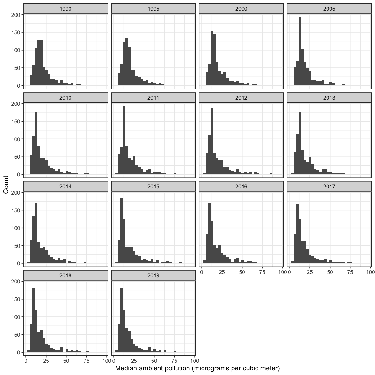
Overview of the lesson
Great, now that we’ve read in the data and practiced plotting, we can start to think about cleaning the data. Remember that our goal is to prepare the ambient pollution data to be compatible with our lung cancer rates so we can directly compare lung cancer rates to ambient pollution levels (we will do this tomorrow). To make this work, we’d like a dataframe that contains columns with the country name, year, and median ambient pollution levels (in micrograms per cubic meter). We will make this comparison for the first year in these datasets, 1990.
What data cleaning do we have to do?
Look back at the three columns in our data object:
location_name,year_id, andug_m3. What might we need to take care of in order to merge these data with our lung cancer rates dataset?Solution
It looks like the
location_namecolumn contains values other than countries, and ouryear_idcolumn has many years, and we are only interested in 1990 for now.
Narrow down rows with filter()
Let’s start by narrowing the dataset to only the year 1990. To do this, we will use the filter() function. Here’s what that looks like:
filter(ambient_pollution_dirty, year_id = 1990)
Error in `filter()`:
! We detected a named input.
ℹ This usually means that you've used `=` instead of `==`.
ℹ Did you mean `year_id == 1990`?
Oops! We got an error, but don’t panic. Error messages are often pretty useful.
In this case, it says that that we used = instead of ==.
That’s because we use = (single equals) when naming arguments that you are passing to functions.
So here R thinks we’re trying to assign 1990 to year, kind of like we do when we’re telling ggplot what we want our aesthetics to be.
What we really want to do is find all of the years that are equal to 1990.
To do this, we have to use == (double equals), which we use when testing if two values are equal to each other:
filter(ambient_pollution_dirty, year_id == 1990)
# A tibble: 690 × 3
location_name year_id ug_m3
<chr> <dbl> <dbl>
1 Global 1990 40.0
2 Southeast Asia, East Asia, and Oceania 1990 41.3
3 East Asia 1990 45.8
4 China 1990 46.4
5 Democratic People's Republic of Korea 1990 39.3
6 Taiwan 1990 21.7
7 Southeast Asia 1990 28.3
8 Cambodia 1990 26.5
9 Indonesia 1990 25.5
10 Lao People's Democratic Republic 1990 25.1
# ℹ 680 more rows
Okay, so it looks like we have 690 observations for the year 1990. Some of these are countries, some are regions of the world, and we have at least one global measurement.
Before we move on, I want to show you a tool called a pipe operator that will be really helpful as we continue. Instead of including the data object as an argument, we can use the pipe operator %>% to pass the data value into the filter function. You can think of %>% as another way to type “and then.”
ambient_pollution_dirty %>% filter(year_id == 1990)
# A tibble: 690 × 3
location_name year_id ug_m3
<chr> <dbl> <dbl>
1 Global 1990 40.0
2 Southeast Asia, East Asia, and Oceania 1990 41.3
3 East Asia 1990 45.8
4 China 1990 46.4
5 Democratic People's Republic of Korea 1990 39.3
6 Taiwan 1990 21.7
7 Southeast Asia 1990 28.3
8 Cambodia 1990 26.5
9 Indonesia 1990 25.5
10 Lao People's Democratic Republic 1990 25.1
# ℹ 680 more rows
This line of code will do the exact same thing as our first summary command, but the piping function tells R to use the ambient_pollution_dirty dataframe as the first argument in the next function.
This lets us “chain” together multiple functions, which will be helpful later. Note that the pipe (%>%) is a bit different from using the ggplot plus (+). Pipes take the output from the left side and use it as input to the right side. In other words, it tells R to do the function on the left and then the function on the right. In contrast, plusses layer on additional information (right side) to a preexisting plot (left side).
We can also add an Enter to make it look nicer:
ambient_pollution_dirty %>%
filter(year_id == 1990)
# A tibble: 690 × 3
location_name year_id ug_m3
<chr> <dbl> <dbl>
1 Global 1990 40.0
2 Southeast Asia, East Asia, and Oceania 1990 41.3
3 East Asia 1990 45.8
4 China 1990 46.4
5 Democratic People's Republic of Korea 1990 39.3
6 Taiwan 1990 21.7
7 Southeast Asia 1990 28.3
8 Cambodia 1990 26.5
9 Indonesia 1990 25.5
10 Lao People's Democratic Republic 1990 25.1
# ℹ 680 more rows
Using the pipe operator %>% and Enter makes our code more readable. The pipe operator %>% also helps to avoid using nested functions and minimizes the need for new variables.
Bonus: Pipe keyboard shortcut
Since we use the pipe operator so often, there is a keyboard shortcut for it in RStudio. You can press Ctrl+Shift+M on Windows or Cmd+Shift+M on a Mac.
Bonus Exercise: Viewing data
Sometimes it can be helpful to explore your data summaries in the View tab. Filter
ambient_pollution_dirtyto only entries from 1990 and use the pipe operator andView()to explore the summary data. Click on the column names to reorder the summary data however you’d like.Solution:
ambient_pollution_dirty %>% filter(year_id == 1990) %>% View()Once you’re done, close out of that window and go back to the window with your code in it.
Bonus Exercise: sorting columns
We just used the View tab to sort our count data, but how could you use code to sort the
ug_m3column? Try to figure it out by searching on the Internet.Solution:
ambient_pollution_dirty %>% filter(year_id == 1990) %>% arrange(desc(ug_m3))# A tibble: 690 × 3 location_name year_id ug_m3 <chr> <dbl> <dbl> 1 Qatar 1990 78.2 2 Niger 1990 70.6 3 Nigeria 1990 69.4 4 India 1990 68.4 5 Egypt 1990 66.1 6 South Asia 1990 65.2 7 South Asia 1990 65.2 8 Cameroon 1990 65.0 9 Mauritania 1990 64.8 10 Nepal 1990 64.0 # ℹ 680 more rowsThe
arrange()function is very helpful for sorting data objects based on one or more columns. Notice we also included the functiondesc(), which tellsarrange()to sort in descending order (largest to smallest).
Great! We’ve managed to reduce our dataset to only the rows corresponding to 1990. Now, the year_id column is obsolete, so let’s learn how to get rid of it.
Subset columns using select()
We use the filter() function to choose a subset of the rows from our data, but when we want to choose a subset of columns from our data we use select(). For example, if we only wanted to see the year (year_id) and median values, we can do:
ambient_pollution_dirty %>%
select(year_id, ug_m3)
# A tibble: 9,660 × 2
year_id ug_m3
<dbl> <dbl>
1 1990 40.0
2 1995 38.9
3 2000 40.6
4 2005 40.6
5 2010 42.7
6 2011 44.4
7 2012 46.1
8 2013 47.1
9 2014 47.3
10 2015 46.1
# ℹ 9,650 more rows
We can also use select() to drop/remove particular columns by putting a minus sign (-) in front of the column name. For example, if we want everything but the year_id column, we can do:
ambient_pollution_dirty %>%
select(-year_id)
# A tibble: 9,660 × 2
location_name ug_m3
<chr> <dbl>
1 Global 40.0
2 Global 38.9
3 Global 40.6
4 Global 40.6
5 Global 42.7
6 Global 44.4
7 Global 46.1
8 Global 47.1
9 Global 47.3
10 Global 46.1
# ℹ 9,650 more rows
Selecting columns
Create a dataframe with only the
location_name, andyear_idcolumns.Solution:
There are multiple ways to do this exercise. Here are two different possibilities.
ambient_pollution_dirty %>% select(location_name, year_id)# A tibble: 9,660 × 2 location_name year_id <chr> <dbl> 1 Global 1990 2 Global 1995 3 Global 2000 4 Global 2005 5 Global 2010 6 Global 2011 7 Global 2012 8 Global 2013 9 Global 2014 10 Global 2015 # ℹ 9,650 more rowsambient_pollution_dirty %>% select(-ug_m3)# A tibble: 9,660 × 2 location_name year_id <chr> <dbl> 1 Global 1990 2 Global 1995 3 Global 2000 4 Global 2005 5 Global 2010 6 Global 2011 7 Global 2012 8 Global 2013 9 Global 2014 10 Global 2015 # ℹ 9,650 more rows
Exercise: use
filter()andselect()to narrow down our dataframe to only thelocation_nameandug_m3for 1990Combine the two functions you have learned so far with the pipe operator to narrow down the dataset to the location names and ambient pollution in the year 1990. Save it to an object called
pollution_1990_dirty.Solution
pollution_1990_dirty <- ambient_pollution_dirty %>% filter(year_id == 1990) %>% select(-year_id)
Great! Now we have our dataset narrowed down and saved to an object.
Checking for duplicate rows
Let’s check to see if our dataset contains duplicate rows. We already know that we have some rows with identical location names, but are the rows identical? We can use the distinct() function, which removes any rows for which all values are duplicates of another row, followed by count() to find out.
Getting distinct columns
Find the number of distinct rows in
pollution_1990_dirtyby piping the data intodistinct()and thencount().Solution:
pollution_1990_dirty %>% distinct() %>% count()# A tibble: 1 × 1 n <int> 1 688
You can see that after applying the distinct() function, our dataset only has 688 rows. This tells us that there are two rows that were exactly identical to other rows in our dataset.
Note that the distinct() function without any arguments checks to see if an entire row is duplicated. We can check to see if there are duplicates in a specific column by writing the column name in the distinct() function. This is helpful if you need to know whether there are multiple rows for some sample ids, for example. Let’s try it here with location name. Before we do, what do you expect to see?
pollution_1990_dirty %>%
distinct(location_name) %>%
count()
# A tibble: 1 × 1
n
<int>
1 685
All right, so we expected at least two rows would be eliminated, because we know there are two rows that are completely identical. But here, we can see that there are up to 5 location_name values with multiple rows, suggesting that some locations may have multiple entries with different values. It’s important to check these out because they might indicate issues with data entry or discordant data.
Grouping and counting rows using group_by() and count()
The group_by() function allows us to treat rows in logical groups defined by categories in at least one column. This will allow us to get summary values for each group. The group_by() function expects you to pass in the name of a column (or multiple columns separated by commas) in your data. When we put it together with count(), we will be able to see how many rows are in each group.
Let’s do this for our pollution_1990_dirty dataset:
pollution_1990_dirty %>%
group_by(location_name) %>%
count()
# A tibble: 685 × 2
# Groups: location_name [685]
location_name n
<chr> <int>
1 Aceh 1
2 Acre 1
3 Afghanistan 1
4 Africa 1
5 African Region 1
6 African Union 1
7 Aguascalientes 1
8 Aichi 1
9 Akershus 1
10 Akita 1
# ℹ 675 more rows
It’s kind of hard to find the ones wth two values. Let’s arrange the counts from highest to lowest using the arrange() function to make it easier to see:
pollution_1990_dirty %>%
group_by(location_name) %>%
count() %>%
arrange(-n)
# A tibble: 685 × 2
# Groups: location_name [685]
location_name n
<chr> <int>
1 Georgia 2
2 North Africa and Middle East 2
3 South Asia 2
4 Stockholm 2
5 Sweden except Stockholm 2
6 Aceh 1
7 Acre 1
8 Afghanistan 1
9 Africa 1
10 African Region 1
# ℹ 675 more rows
Note that you might get a message about the summarize function regrouping the output by ‘location_name’. This simply indicates what the function is grouping by.
We can also group by multiple variables. We’ll do more with this later. Now, we know which locations have multiple entries - but what if we want to look at them?
Review: Filtering to specific location names
Break into your groups of two and choose a location name that has multiple entries. Filter
pollution_1990_dirtyto look at those entries in the dataset.Example solution:
pollution_1990_dirty %>% filter(location_name == "Georgia")# A tibble: 2 × 2 location_name ug_m3 <chr> <dbl> 1 Georgia 17.9 2 Georgia 15.1
Now, we want to clean these data up so there is only one row per location. To do that, we will need to add a new column with revised pollution levels.
Make new variables with mutate()
The function we use to create new columns is called mutate(). Let’s go ahead and take care of the location_names which have two different median pollution values by making a new column called pollution that is the mean of ug_m3. We can then remove the ug_m3 column and store the resulting data object as pollution_1990.
pollution_1990 <- pollution_1990_dirty %>%
group_by(location_name) %>%
mutate(pollution = mean(ug_m3)) %>%
select(-ug_m3) %>%
distinct()
You can see that pollution_1990 has 685 rows, as we expect, since we took care of the duplicated location_names.
Note: here, we took the mean to take care of duplicates and multiple entries, but this is not always the best way to do so. When working with your own data, make sure to think carefully about your dataset, what these multiple entries really mean, and whether you want to leave them as they are or take care of them in some different way.
Bonus Exercise: Check to see if all rows are distinct
Do we have any duplicated rows in our pollution_1990 dataset now? HINT: You might get an unexpected result. Look at the code we used to make pollution_1990 to try to figure out why.
Example solution:
pollution_1990 %>% distinct() %>% count()# A tibble: 685 × 2 # Groups: location_name [685] location_name n <chr> <int> 1 Aceh 1 2 Acre 1 3 Afghanistan 1 4 Africa 1 5 African Region 1 6 African Union 1 7 Aguascalientes 1 8 Aichi 1 9 Akershus 1 10 Akita 1 # ℹ 675 more rowsHmm that’s not like the counts we’ve gotten before. That’s because our dataframe is still grouped by
location_name. Here, we actually took distinct rows for each group. In actuality, we want distinct rows for the entire dataset (which should be the same thing since each group is unique). To get the output we want, we can use theungroup()function before callingdistinct():pollution_1990 %>% ungroup() %>% distinct() %>% count()# A tibble: 1 × 1 n <int> 1 685Since the number of rows in pollution_1990 is equal to the number of rows after calling distinct, this means we no longer have any distinct rows in our dataset.
Joining dataframes
Now we’re almost ready to join our pollution data to the smoking and lung cancer data. Let’s read in our smoking_cancer_1990.csv and save it to an object called smoking_1990.
smoking_1990 <- read_csv("data/smoking_cancer_1990.csv")
Rows: 191 Columns: 6
── Column specification ────────────────────────────────────────────────────────
Delimiter: ","
chr (2): country, continent
dbl (4): year, pop, smoke_pct, lung_cancer_pct
ℹ Use `spec()` to retrieve the full column specification for this data.
ℹ Specify the column types or set `show_col_types = FALSE` to quiet this message.
Look at the data in pollution_1990 and smoking_1990. If you had to merge these two dataframes together, which columns would you use to merge them together? If you said location_name and country, you’re right! But before we join the datasets, we need to make sure these columns are named the same thing.
Re-naming columns
Rename the
location_namecolumn tocountryin thepollution_1990dataset. Store in an object calledpollution_1990_clean. HINT: The function you want is part of thedplyrpackage. Try to guess what the name of the function is, and if you’re having trouble try searching for it on the Internet.Solution:
pollution_1990_clean <- pollution_1990 %>% rename(country = location_name)Note that the column is labeled
countryeven though it has values beyond the names of countries. We will take care of this later when we join datasets.
Because the country column is now present in both datasets, we’ll call country our “key”. We want to match the rows in each dataframe together based on this key. Note that the values within the country column have to be exactly identical for them to match (including the same case).
What problems might we run into with merging?
Solution
We might not have pollution data for all of the countries in the
smoking_1990dataset and vice versa. Also, a country might be represented in both dataframes but not by the same name in both places.
The dplyr package has a number of tools for joining dataframes together depending on what we want to do with the rows of the data of countries that are not represented in both dataframes. Here we’ll be using left_join().
In a “left join”, the new dataframe only has those rows for the key values that are found in the first dataframe listed. This is a very commonly used join.
Bonus: Other dplyr join functions
Other joins and can be performed using
inner_join(),right_join(),full_join(), andanti_join(). In a “left join”, if the key is present in the left hand dataframe, it will appear in the output, even if it is not found in the the right hand dataframe. For a right join, the opposite is true. For a full join, all possible keys are included in the output dataframe. For an anti join, only ones found in the left data frame are included.Image source
Let’s give the left_join() function a try. We will put our smoking_1990 dataset on the left so that we maintain all of the rows we had in that dataset.
left_join(smoking_1990, pollution_1990_clean)
Joining with `by = join_by(country)`
# A tibble: 191 × 7
year country continent pop smoke_pct lung_cancer_pct pollution
<dbl> <chr> <chr> <dbl> <dbl> <dbl> <dbl>
1 1990 Afghanistan Asia 1.24e7 3.12 0.0127 46.2
2 1990 Albania Europe 3.29e6 24.2 0.0327 23.8
3 1990 Algeria Africa 2.58e7 18.9 0.0118 29.4
4 1990 Andorra Europe 5.45e4 36.6 0.0609 13.4
5 1990 Angola Africa 1.18e7 12.5 0.0139 27.7
6 1990 Antigua and Barbu… North Am… 6.25e4 6.80 0.0105 16.2
7 1990 Argentina South Am… 3.26e7 30.4 0.0344 14.8
8 1990 Armenia Europe 3.54e6 30.5 0.0441 30.0
9 1990 Australia Oceania 1.71e7 29.3 0.0599 7.13
10 1990 Austria Europe 7.68e6 35.4 0.0439 20.3
# ℹ 181 more rows
We now have data from both datasets joined together in the same dataframe. Notice that the number of rows here, 191, is the same as the number of rows in the smoking_1990 dataset? One thing to note about the output is that left_join() tells us that that it joined by “country”.
Alright, let’s explore this joined data a little bit.
Checking for missing values
First, let’s check for any missing values. We will start by using the drop_na() function, which is a tidyverse function that removes any rows that have missing values. Then we will check the number of rows in our dataset using count() and compare to the original to see if we lost any rows with missing data.
left_join(smoking_1990, pollution_1990_clean) %>%
drop_na() %>%
distinct() %>%
count()
Joining with `by = join_by(country)`
# A tibble: 1 × 1
n
<int>
1 189
It looks like the dataframe has 189 rows after we drop any observations with missing values. This means there are two rows with missing values.
Note that since we used left_join, we expect all the data from the smoking_2019 dataset to be there, so if we have missing values, they will be in the pollution column. We will look for rows with missing values in the pollution column using the filter() function and is.na(), which is helpful for identifying missing data
left_join(smoking_1990, pollution_1990_clean) %>%
filter(is.na(pollution))
Joining with `by = join_by(country)`
# A tibble: 2 × 7
year country continent pop smoke_pct lung_cancer_pct pollution
<dbl> <chr> <chr> <dbl> <dbl> <dbl> <dbl>
1 1990 Slovak Republic Europe 5299187 33.7 0.0699 NA
2 1990 Vietnam Asia 67988855 29.4 0.0216 NA
We can see that were missing pollution data for Vietnam and Slovak Republic. Note that we were expecting two rows with missing values, and we found both of them! That’s great news.
If we look at the pollution_1990_clean data by clicking on it in the environment and sort by country, we can see that Vientam and Slovak Republic are called different things in the pollution_1990_clean dataframe. They’re called “Viet Nam” and “Slovakia,” respectively. Using mutate() and case_when(), we can update the pollution_2019 data so that the country names for Vietnam and Slovak Republic match those in the smoking_1990 data. case_when() is a super useful function that uses information from a column (or columns) in your dataset to update or create new columns.
Let’s use case_when() to change “Viet Nam” to “Vietnam”.
pollution_1990_clean %>%
mutate(country = case_when(country == "Viet Nam" ~ "Vietnam",
TRUE ~ country))
# A tibble: 685 × 2
# Groups: country [685]
country pollution
<chr> <dbl>
1 Global 40.0
2 Southeast Asia, East Asia, and Oceania 41.3
3 East Asia 45.8
4 China 46.4
5 Democratic People's Republic of Korea 39.3
6 Taiwan 21.7
7 Southeast Asia 28.3
8 Cambodia 26.5
9 Indonesia 25.5
10 Lao People's Democratic Republic 25.1
# ℹ 675 more rows
Practicing
case_when()Starting with the code we wrote above, add to it to change “Slovakia” to “Slovak Republic”.
One possible solution:
pollution_1990_clean %>% mutate(country = case_when(country == "Viet Nam" ~ "Vietnam", country == "Slovakia" ~ "Slovak Republic", TRUE ~ country))# A tibble: 685 × 2 # Groups: country [685] country pollution <chr> <dbl> 1 Global 40.0 2 Southeast Asia, East Asia, and Oceania 41.3 3 East Asia 45.8 4 China 46.4 5 Democratic People's Republic of Korea 39.3 6 Taiwan 21.7 7 Southeast Asia 28.3 8 Cambodia 26.5 9 Indonesia 25.5 10 Lao People's Democratic Republic 25.1 # ℹ 675 more rows
Checking to see if our code worked
Starting with the code we wrote above, add or modify it see if it worked the way we want it to - did we change “Viet Nam” to “Vietnam” and “Slovakia” to “Slovak Republic” while keeping everything else the same?
One possible solution:
pollution_1990_clean %>% mutate(country_new = case_when(country == "Viet Nam" ~ "Vietnam", country == "Slovakia" ~ "Slovak Republic", TRUE ~ country)) %>% filter(country != country_new)# A tibble: 2 × 3 # Groups: country [2] country pollution country_new <chr> <dbl> <chr> 1 Viet Nam 25.6 Vietnam 2 Slovakia 26.1 Slovak Republic
Once we’re sure that our code is working correctly, let’s save this to pollution_2019_clean.
pollution_1990_clean <- pollution_1990_clean %>%
mutate(country = case_when(country == "Viet Nam" ~ "Vietnam",
country == "Slovakia" ~ "Slovak Republic",
TRUE ~ country))
IMPORTANT: Here, we overwrote our pollution_2019_clean dataframe. In other words, we replaced the existing data object with a new one. This is generally NOT recommended practice, but is often needed when first performing exploratory data analysis as we are here. After you finish exploratory analysis, it’s always a good idea to go back and clean up your code to avoid overwriting objects.
Bonus Exercise: Cleaning up code
How would you clean up your code to avoid overwriting
pollution_2019_cleanas we did above? Hint: start with the pollution_1990 dataframe. Challenge: Start at the very beginning, from reading in your data, and clean it all in one big step (this is what we do once we’ve figured out how we want to clean our data - we then clean up our code).Solution:
pollution_1990_clean <- pollution_1990 %>% rename(country = location_name) %>% mutate(country = case_when(country == "Viet Nam" ~ "Vietnam", country == "Slovakia" ~ "Slovak Republic", TRUE ~ country))Challenge solution:
pollution_1990_clean <- read_csv("data/ambient_pollution.csv") %>% filter(year_id == 1990) %>% select(-year_id) %>% group_by(location_name) %>% mutate(pollution = mean(ug_m3)) %>% ungroup() %>% select(-ug_m3) %>% distinct() %>% rename(country = location_name) %>% mutate(country = case_when(country == "Viet Nam" ~ "Vietnam", country == "Slovakia" ~ "Slovak Republic", TRUE ~ country))Rows: 9660 Columns: 3 ── Column specification ──────────────────────────────────────────────────────── Delimiter: "," chr (1): location_name dbl (2): year_id, ug_m3 ℹ Use `spec()` to retrieve the full column specification for this data. ℹ Specify the column types or set `show_col_types = FALSE` to quiet this message.
Alright, now let’s left_join() our dataframes again and filter for missing values to see how it looks.
left_join(smoking_1990, pollution_1990_clean) %>%
filter(is.na(pollution))
Joining with `by = join_by(country)`
# A tibble: 0 × 7
# ℹ 7 variables: year <dbl>, country <chr>, continent <chr>, pop <dbl>,
# smoke_pct <dbl>, lung_cancer_pct <dbl>, pollution <dbl>
Now you can see that we have an empty dataframe! That’s great news; it means that we do not have any rows with missing pollution data.
Finally, let’s use left_join() to create a new dataframe:
smoking_pollution <- left_join(smoking_1990, pollution_1990_clean)
Joining with `by = join_by(country)`
We have reached our data cleaning goal! One of the best aspects of doing all of these steps coded in R is that our efforts are reproducible, and the raw data is maintained. With good documentation of data cleaning and analysis steps, we could easily share our work with another researcher who would be able to repeat what we’ve done. However, it’s also nice to have a saved csv copy of our clean data. That way we can access it later without needing to redo our data cleaning, and we can also share the cleaned data with collaborators. To save our dataframe, we’ll use write_csv().
write_csv(smoking_pollution, "data/smoking_pollution.csv")
Great - Now our data is ready to analyze tomorrow!
Applying it to your own data
Now that we’ve learned how clean data, it’s time to read in, clean, and make plots with your own data! Use your ideas from your brainstorming session yesterday to help you get started, but feel free to branch out and explore other things as well. Let us know if you have questions; we’re here to help.
- Make sure you have your R project opened in R Studio.
- Open a new file in R and save it with an informative name.
- Read in your data.
- Explore your data and clean as needed.
- What did you identify that you have to address before you can start analyzing the data?
- e.g. missing data, column names with spaces, columns with both numbers and characters
- What did you identify that you have to address before you can start analyzing the data?
- Create at least 3 plots of your data that help answer the questions you posed yesterday.
Answer the questions below as you go through these steps.
- What did you learn as you explored your data? Did you have to modify your questions, and if so, why and how?
- What did you have to do to clean your data?
- What plots did you work on that relate to your questions of interest?
Glossary of terms
- Pipe (
%>%): takes input (before pipe) and then performs next step (after pipe). filter(): keeps only certain rows.select(): keeps only certain columns.group_by(): groups rows by a certain column.mutate(): makes new columns.count(): counts rows; if grouped, counts within groups.drop_na(): removes any rows with NA values.duplicated(): removes any rows that are entirely duplicated.left_join(): joins two dataframes by common column names, keeps all rows in left dataframe.case_when(): uses information from columns to update/create a columnwrite_csv(): saves dataframe to a csv file.
Key Points
Package loading is an important first step in preparing an R environment.
Assessing data source and structure is an important first step in analysis.
There are many useful functions in the
tidyversepackages that can aid in data analysis.Preparing data for analysis can take significant effort and planning.
R for Data Analysis
Overview
Teaching: 75 min
Exercises: 15 minQuestions
How can I summarise my data in R?
How can R help make my research more reproducible?
Objectives
To become familiar with the functions of the
dplyrandtidyrpackages.To be able to create plots and summary tables to answer analysis questions.
Contents
- Day 2 review
- Overview of the lesson
- Get stats fast with
summarise() - Plotting for exploratory data analysis
- [Bonus content] (#bonus-content)
- Calculating percentages
- Changing the shape of the data
- Plotting wide data
- Additional practice
- Applying it to your own data
Day 2 review
Yesterday we learned all about data cleaning, but we didn’t cover everything.
- Make a list of what we learned yesterday related to data cleaning.
- Make a list of things we didn’t learn yesterday that you sometimes have to do while data cleaning.
- Choose one item from the list of things we didn’t learn and use the Internet to search for a way to do it using the
tidyverse.
Overview of the lesson
So far, you’ve learned how to load, plot, merge, and clean data. In the process, you’ve learned a lot of new functions which are useful for transforming data. Today, we are going to put all those new skills you learned together and learn a few new functions that will be really helpful for exploratory data analysis. We’ll start with a few examples of how plotting can be a really useful tool for exploratory data analysis. Then, we’ll learn a function that will help us get summary statistics for our data and compare those summary statistics to plots. We’ll also learn how to calculate proportions and percentages. Finally, we’ll learn how to change the shape of data to make certain analyses more straight forward. First, let’s read in the data on smoking, lung cancer rates, and pollution that we generated yesterday:
library(tidyverse)
Warning: package 'ggplot2' was built under R version 4.3.3
Warning: package 'tibble' was built under R version 4.3.3
Warning: package 'purrr' was built under R version 4.3.3
Warning: package 'lubridate' was built under R version 4.3.3
── Attaching core tidyverse packages ──────────────────────── tidyverse 2.0.0 ──
✔ dplyr     1.1.4     ✔ readr     2.1.5
✔ forcats   1.0.0     ✔ stringr   1.5.1
✔ ggplot2   3.5.2     ✔ tibble    3.3.0
✔ lubridate 1.9.4     ✔ tidyr     1.3.1
✔ purrr     1.0.4
── Conflicts ────────────────────────────────────────── tidyverse_conflicts() ──
✖ dplyr::filter() masks stats::filter()
✖ dplyr::lag()    masks stats::lag()
ℹ Use the conflicted package (<http://conflicted.r-lib.org/>) to force all conflicts to become errors
smoking_pollution <- read_csv("data/smoking_pollution.csv")
Rows: 191 Columns: 7
── Column specification ────────────────────────────────────────────────────────
Delimiter: ","
chr (2): country, continent
dbl (5): year, pop, smoke_pct, lung_cancer_pct, pollution

ℹ Use `spec()` to retrieve the full column specification for this data.
ℹ Specify the column types or set `show_col_types = FALSE` to quiet this message.
Get stats fast with summarise()
Let’s say we would like to know the mean (average) smoking rate in the dataset. R has a built in function function called mean() that will calculate this value for us. We can apply that function to our smoke_pct column using the summarise() function. Here’s what that looks like:
smoking_pollution %>%
    summarise(mean_smoke_pct = mean(smoke_pct))
# A tibble: 1 × 1
  mean_smoke_pct
           <dbl>
1           23.9
When we call summarise(), we can use any of the column names of our data object as values to pass to other functions. summarise() will return a new data object and our value will be returned as a column.
Note: The
summarise()andsummarise()functions perform identical functions.
The mean_smoke_pct= part tells summarise() to use “mean_smoke_pct” as the name of the new column. Note that you don’t have to have quotes around this new name as long as it starts with a letter and doesn’t include a space.
When you call summarise(), you can also create more than one new column. To do so, you must separate your columns with a comma. Building on the code from above, let’s add a new column that calculates the minimum and maximum percent of smokers.
smoking_pollution %>%
  summarise(mean_smoke_pct=mean(smoke_pct),
            min_smoke_pct=min(smoke_pct),
            max_smoke_pct=max(smoke_pct))
# A tibble: 1 × 3
  mean_smoke_pct min_smoke_pct max_smoke_pct
           <dbl>         <dbl>         <dbl>
1           23.9          3.12          46.9
Perhaps one of the most powerful ways to use summarise() is to combine it with group_by(). This enables you to calculate summary statistics for specific groups. For example, suppose we wanted to calculate the the mean, min, and max smoke_pct for each continent. How would you modify the code above?
smoking_pollution %>%
    group_by(continent) %>%
    summarise(mean_smoke_pct=mean(smoke_pct),
            min_smoke_pct=min(smoke_pct),
            max_smoke_pct=max(smoke_pct))
# A tibble: 6 × 4
  continent     mean_smoke_pct min_smoke_pct max_smoke_pct
  <chr>                  <dbl>         <dbl>         <dbl>
1 Africa                  15.0          3.81          31.9
2 Asia                    25.1          3.12          39.7
3 Europe                  34.2         21.8           46.1
4 North America           16.1          6.55          33.1
5 Oceania                 33.3         21.2           46.9
6 South America           24.4          8.33          39.5
Exercise: Summary stats and boxplots
Part 1: Use
group_by()andsummarise()to find the median, min, max, and interquartile range oflung_cancer_pctfor each continent.Part 2: Make a box plot of
pollutionon the y axis and continent on the x axis. Compare your plot to your table. What do you notice? Which do you think is easier to interpret?Solution
Part 1: Use
group_by()andsummarise()to find the median, min, max, and interquartile range ofpollutionfor each continent.smoking_pollution %>% group_by(continent) %>% summarise(med_pollution = median(pollution), min_pollution = min(pollution), max_pollution = max(pollution), iqr_pollution = IQR(pollution))# A tibble: 6 × 5 continent med_pollution min_pollution max_pollution iqr_pollution <chr> <dbl> <dbl> <dbl> <dbl> 1 Africa 35.7 14.2 70.6 24.1 2 Asia 29.4 7.63 78.2 22.4 3 Europe 19.6 6.81 43.7 9.69 4 North America 18.5 8.14 38.1 4.64 5 Oceania 8.05 4.69 14.3 2.45 6 South America 20.2 9.97 45.3 12.2Part 2: Make a box plot of
pollutionon the y axis and continent on the x axis. Compare your plot to your table. What do you notice?smoking_pollution %>% ggplot(aes(x = continent, y = pollution)) + geom_boxplot()
When comparing your table to your plot, you’ll notice that the dark horizontal lines represent median values. The boxes have lengths equal to the interquartile range (IQR). And the highest and lowest values for each continent match the table as well. The plot makes it easier to see differences between continents. The table provides finer details for comparison. What you choose to report will depend on whether you want to bring attention to those finer details or whether you want to discuss overall trends.
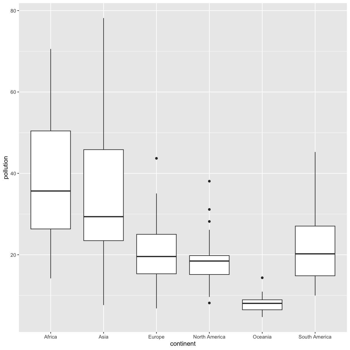
Plotting for exploratory data analysis
For our analysis, we have three questions we’d like to answer:
- Is there a relationship between population and ambient pollution levels (in micrograms per cubic meter)?
- Which continent has the highest pollution levels per capita?
- Is there a relationship between ambient pollution levels per capita and lung cancer rates?
1) Is there a relationship between population and ambient pollution levels (in micrograms per cubic meter)?
To answer this question, we’ll plot ambient pollution levels against population using a scatter plot. It will help to scale the x axis (population) log 10.
smoking_pollution %>%
  ggplot(aes(x = pop, y = pollution)) +
  geom_point() +
  scale_x_log10() +
  labs(x = "Population", y = "Ambient pollution levels (micrograms/cubic meter)",
       size = "Population\n(millions)") +
  theme_bw()
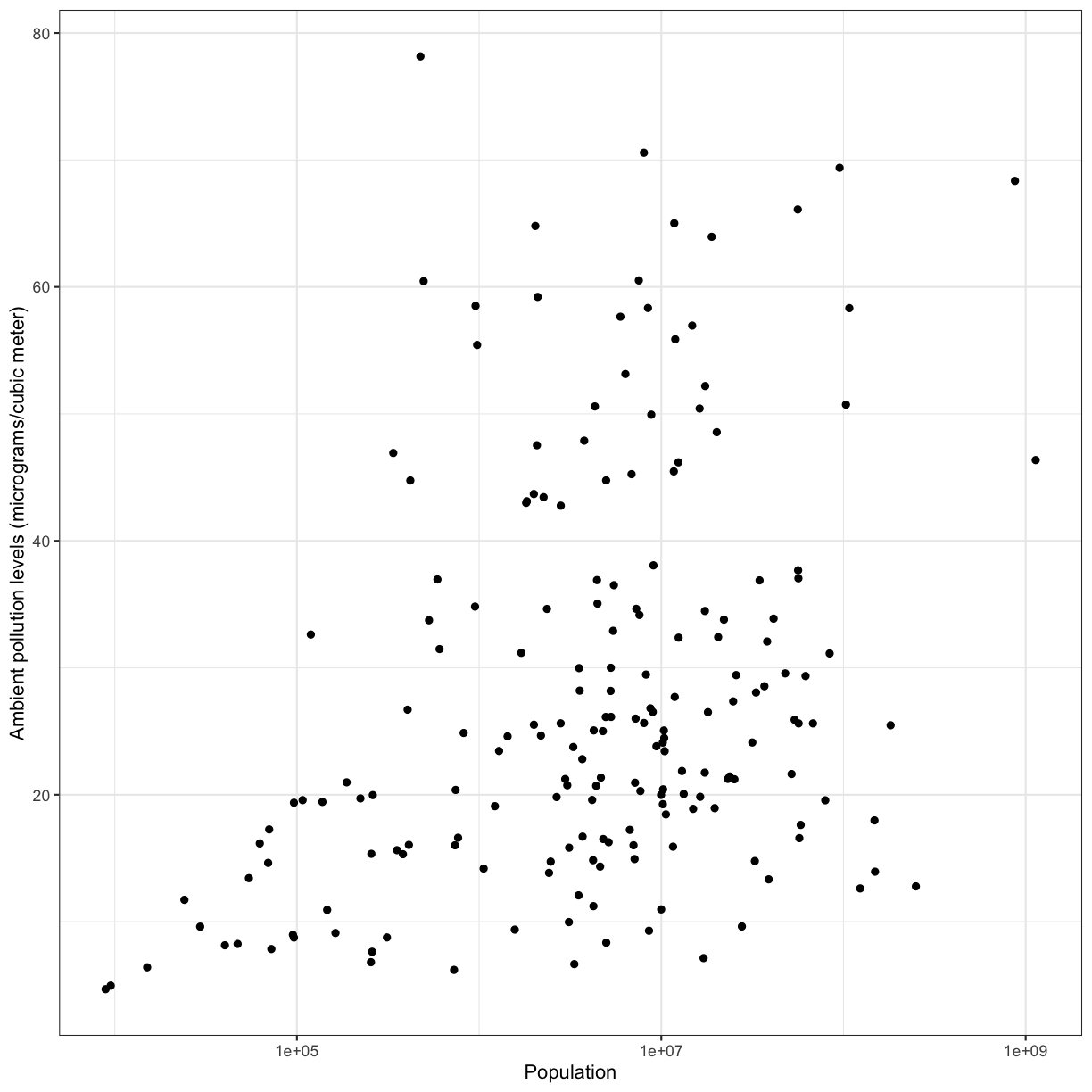
We observe a positive association between ambient pollution levels and population.
To help clarify the association, we can add a fit line through the data using geom_smooth(method = "lm"). Notice we added the method = "lm" argument. This tells geom_smooth() that we would like a linear model (lm) fit to the data.
smoking_pollution %>%
  ggplot(aes(x = pop, y = pollution)) +
  geom_point() +
  geom_smooth(method = "lm") +
  scale_x_log10() +
  labs(x = "Population", y = "Ambient pollution levels (micrograms/cubic meter)", size = "Population\n(millions)") +
  theme_bw()
`geom_smooth()` using formula = 'y ~ x'
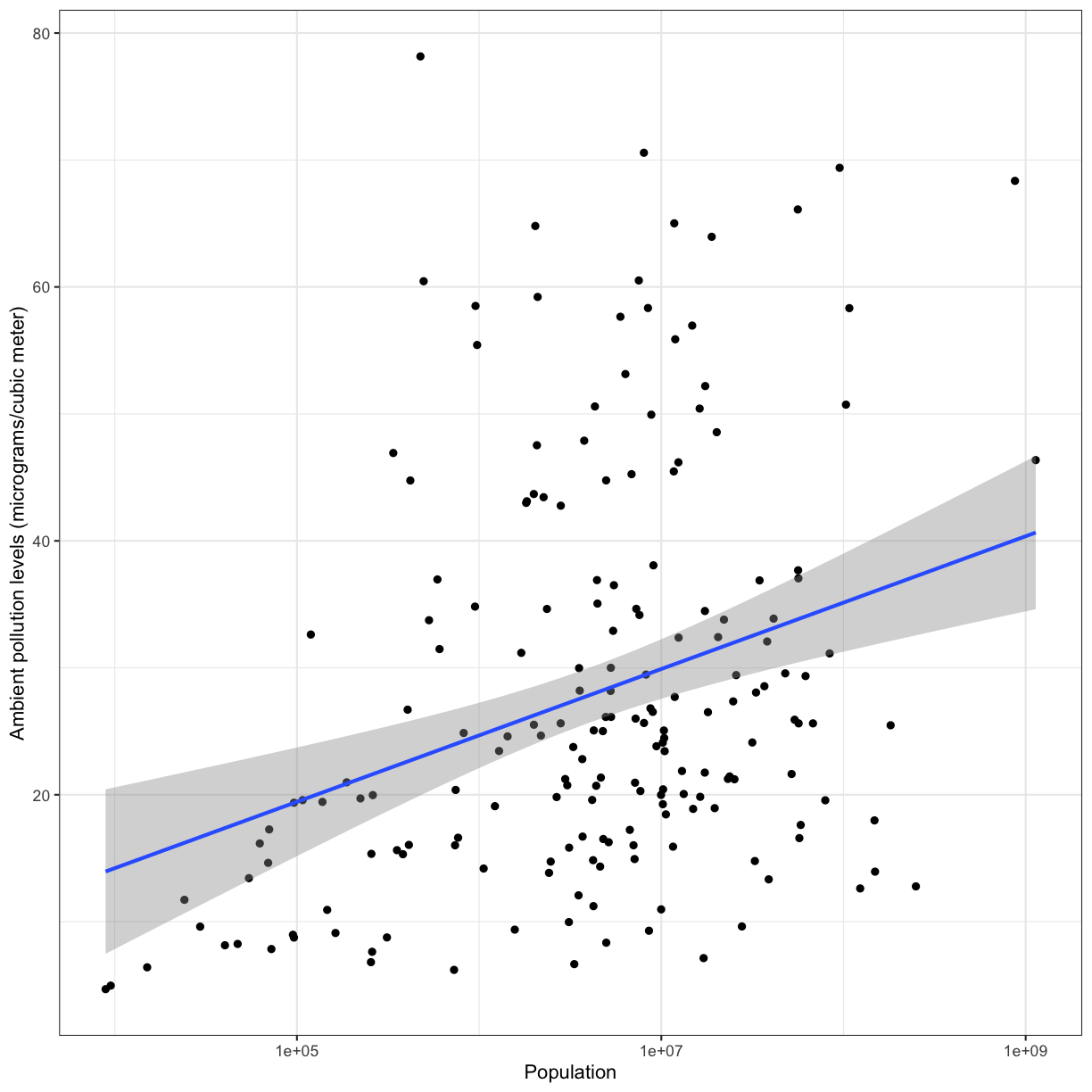
To answer our first question, we observe a positive association between population and ambient pollution. In other words, countries with higher populations tend to have higher ambient pollution levels. It is very important to remember that associations are not indicative of causality and there could be confounding variables that may be playing into this apparent relationship. Can you think of any confounding factors we haven’t accoutned for?
Challenge: 2) which continent has the highest pollution levels per capita?
To answer this question, we need to calculate the pollution levels per capita for each country using
mutate(). Then plot a boxplot to look at these levels by continent. Hint: it may help to scale the y axis log10Solution:
smoking_pollution %>%
  mutate(pollution_capita = pollution/pop) %>%
  ggplot(aes(x = continent, y = pollution_capita)) +
  geom_boxplot() +
  scale_y_log10() +
  labs(y = "Pollution (micrograms/cubic meter) per capita")+
  theme_bw()
Which continent has the highest pollution levels per capita? What other factors do you think could be driving this observation?
Challenge: 3) Is there a relationship between ambient pollution levels per capita and lung cancer rates?
To answer this question, let’s make a scatter plot with ambient pollution levels on the x axis and lung cancer rates on the y axis. Hint: Make sure to scale the x-axis log10.
Solution:
smoking_pollution %>%
  mutate(pollution_capita = pollution/pop) %>%
  ggplot(aes(x = pollution_capita, y = lung_cancer_pct)) +
  geom_point() +
  scale_x_log10() +
  labs(x = "Pollution (micrograms/cubic meter) per capita", y = "Percent of people with lung cancer")+
  theme_bw()
There does not appear to be a direct relationship between pollution and lung cancer rates.
Bonus content
Calculating percentages
Finding percentages using dplyr can be a little bit complicated. However, it’s a very useful skill! We’ve included an exercise here that provides an example for how to calculate percentages.
Percentages
What percentage of the global population in 1990 did Africa make up? What percentage of the population in Africa did Kenya make up?
Solution
Create a new variable using
group_by()andmutate()that calculates percentages for the pop variable.smoking_pollution %>% mutate(total_pop = sum(pop)) %>% #total_pop is the global population group_by(continent) %>% #grouping by continent allows us to calculate the population on each continent mutate(cont_pop = sum(pop), #cont_pop is the continental population cont_percent = cont_pop/total_pop * 100, #cont_percent is the percent of the global population for the continent country_cont_pct = pop/cont_pop * 100) %>% #country_cont_pct is the percent of the continent population for a given country select(country, continent, cont_percent, country_cont_pct) %>% filter(country == "Kenya")# A tibble: 1 × 4 # Groups: continent [1] country continent cont_percent country_cont_pct <chr> <chr> <dbl> <dbl> 1 Kenya Africa 12.1 3.77This table shows that Kenya makes up 4% of the population of Africa, and Africa makes up 12% of the global population.
Changing the shape of the data
Data comes in many shapes and sizes, and one way we classify data is either “wide” or “long.” Data that is “long” has one row per observation. The smoking data is in a long format. We have one row for each country for each year and each different measurement for that country is in a different column. We might describe this data as “tidy” because it makes it easy to work with ggplot2 and dplyr functions (this is where the “tidy” in “tidyverse” comes from). As tidy as it may be, sometimes we may want our data in a “wide” format. Typically in “wide” format each row represents a group of observations and each value is placed in a different column rather than a different row. For example, let’s read in a smoking and lung cancer data set that covers many years and take a look at it:
smoking_cancer <- read_csv("data/smoking_cancer.csv")
Rows: 5719 Columns: 6
── Column specification ────────────────────────────────────────────────────────
Delimiter: ","
chr (2): country, continent
dbl (4): year, pop, smoke_pct, lung_cancer_pct

ℹ Use `spec()` to retrieve the full column specification for this data.
ℹ Specify the column types or set `show_col_types = FALSE` to quiet this message.
It has one row for each country for each year the data were collected. But maybe we want only one row per country and want to spread the percent of smokers values into different columns (one for each year).
The tidyr package contains the functions pivot_wider() and pivot_longer() that make it easy to switch between the two formats. The tidyr package is included in the tidyverse package so we don’t need to do anything to load it.
Let’s create a wide version of our data using pivot_wider():
smoking_cancer %>%
  group_by(country, continent, year) %>%
  summarise(smoke_pct = mean(smoke_pct)) %>%
  pivot_wider(names_from = year, values_from = smoke_pct)
`summarise()` has grouped output by 'country', 'continent'. You can override
using the `.groups` argument.
# A tibble: 191 × 32
# Groups:   country, continent [191]
   country     continent `1990` `1991` `1992` `1993` `1994` `1995` `1996` `1997`
   <chr>       <chr>      <dbl>  <dbl>  <dbl>  <dbl>  <dbl>  <dbl>  <dbl>  <dbl>
 1 Afghanistan Asia        3.12   3.29   3.53   3.77   4.00   4.25   4.53   4.82
 2 Albania     Europe     24.2   24.1   24.0   24.0   23.9   23.8   23.8   23.9
 3 Algeria     Africa     18.9   18.7   18.6   18.4   18.2   18.0   17.8   17.6
 4 Andorra     Europe     36.6   36.5   36.3   36.2   35.9   35.5   35.2   34.9
 5 Angola      Africa     12.5   12.4   12.2   12.0   11.8   11.5   11.3   11.0
 6 Antigua an… North Am…   6.80   6.94   7.06   7.17   7.27   7.36   7.43   7.47
 7 Argentina   South Am…  30.4   30.1   29.9   29.7   29.5   29.4   29.2   29.1
 8 Armenia     Europe     30.5   30.4   30.2   30.0   29.9   29.7   29.6   29.5
 9 Australia   Oceania    29.3   28.8   28.4   27.9   27.5   27.0   26.4   25.9
10 Austria     Europe     35.4   35.8   36.2   36.6   37.0   37.4   37.8   38.1
# ℹ 181 more rows
# ℹ 22 more variables: `1998` <dbl>, `1999` <dbl>, `2000` <dbl>, `2001` <dbl>,
#   `2002` <dbl>, `2003` <dbl>, `2004` <dbl>, `2005` <dbl>, `2006` <dbl>,
#   `2007` <dbl>, `2008` <dbl>, `2009` <dbl>, `2010` <dbl>, `2011` <dbl>,
#   `2012` <dbl>, `2013` <dbl>, `2014` <dbl>, `2015` <dbl>, `2016` <dbl>,
#   `2017` <dbl>, `2018` <dbl>, `2019` <dbl>
Notice here that we tell pivot_wider() which columns to pull the names we wish our new columns to be named from the year variable, and the values to populate those columns from the smoke_pct variable. (Again, neither of which have to be in quotes in the code when there are no special characters or spaces - certainly an incentive not to use special characters or spaces!) We see that the resulting table has new columns by year, and the values populate it with our remaining variables dictating the rows.
Plotting wide data
Let’s make a plot with our wide data comparing percent of smokers in 1990 to percent of smokers in 2010 to see how it has changed for each country.
smoking_cancer %>%
  group_by(country, continent, year) %>%
  summarise(smoke_pct = mean(smoke_pct)) %>%
  pivot_wider(names_from = year, values_from = smoke_pct) %>%
  ggplot(aes(x = 1990, y = 2010)) +
  geom_point()
`summarise()` has grouped output by 'country', 'continent'. You can override
using the `.groups` argument.
Warning in geom_point(): All aesthetics have length 1, but the data has 191 rows.
ℹ Please consider using `annotate()` or provide this layer with data containing
  a single row.
Hmm that’s not what we want. ggplot just plotted the numbers 1990 and 2010 instead of the data from the years. That’s because it evaluates those as numbers instead of column names. To fix this, we can add a prefix to the years in pivot_wider():
smoking_cancer %>%
  group_by(country, continent, year) %>%
  summarise(smoke_pct = mean(smoke_pct)) %>%
  pivot_wider(names_from = year, values_from = smoke_pct, names_prefix = 'y') %>%
  ggplot(aes(x = y1990, y = y2010)) +
  geom_point()
`summarise()` has grouped output by 'country', 'continent'. You can override
using the `.groups` argument.
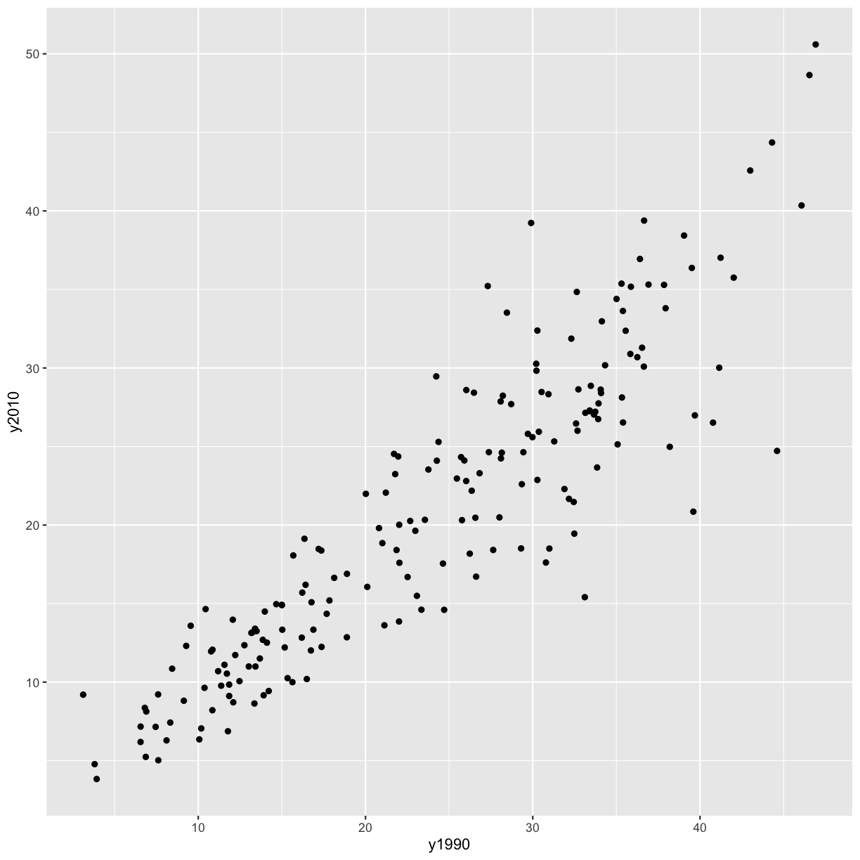
Alright, now we have a plot with the mean percent of smokers in in 1990 on the x axis and the mean percent of smokers in 2010 on the y axis, and each point represents a country. However, the different ranges on the x and y axis make it hard to compare the points. Let’s fix that by adding a line at y=x.
smoking_cancer %>%
  group_by(country, continent, year) %>%
  summarise(smoke_pct = mean(smoke_pct)) %>%
  pivot_wider(names_from = year, values_from = smoke_pct, names_prefix = 'y') %>%
  ggplot(aes(x = y1990, y = y2010)) +
  geom_point() +
  geom_abline(intercept = 0, slope = 1)
`summarise()` has grouped output by 'country', 'continent'. You can override
using the `.groups` argument.
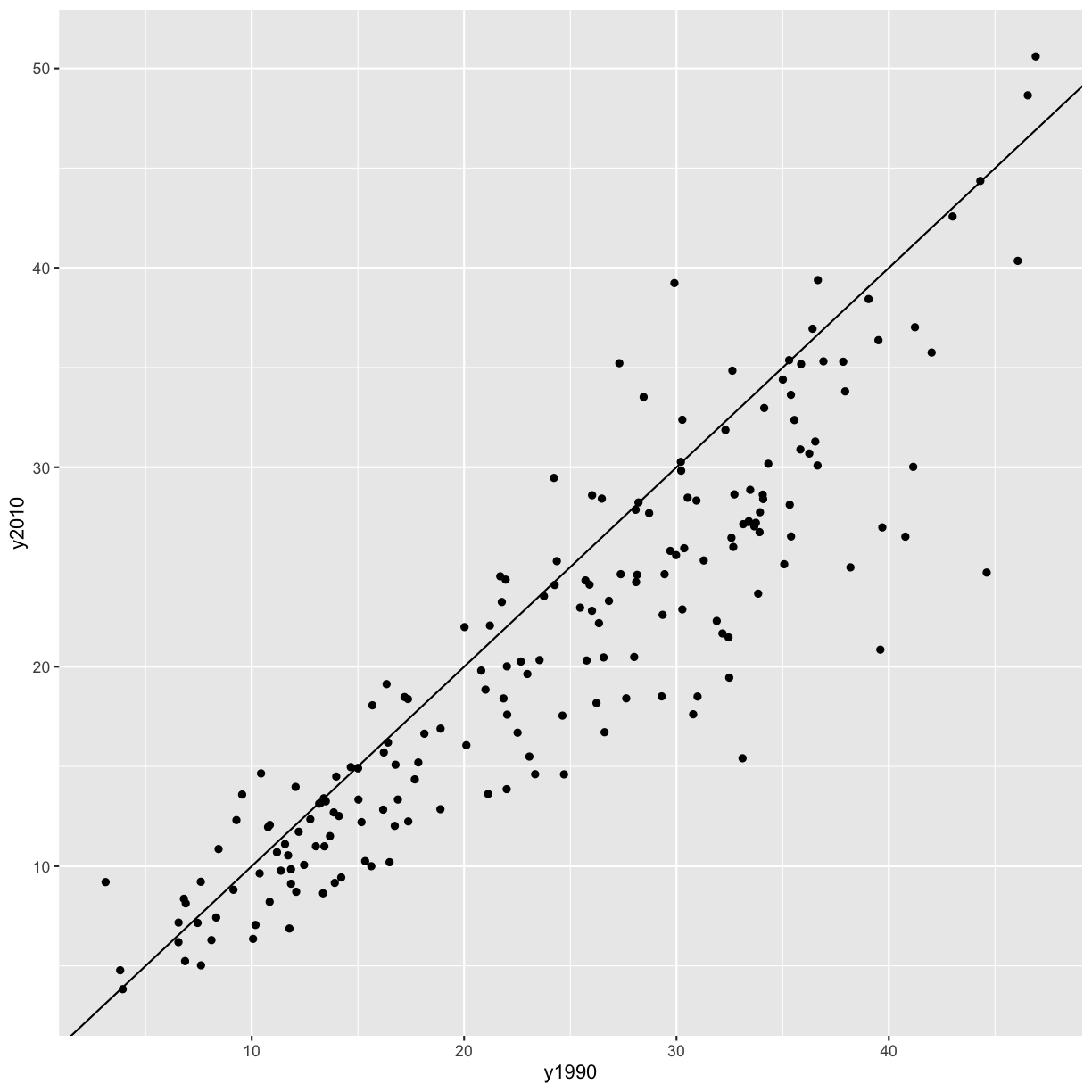
It seems like in most countries the percent of smokers has decreased from 1990 to 2010, since most of the points fall below the line y = x. However, there are some countries where smoking has increased (i.e. the points are above the line y = x). Let’s figure out which those are!
Bonus: Identifying countries with more smokers in 2010 than 1990
Use what you’ve learned from today to figure out which countries had higher smoking percentage in 2010 than 1990.
Bonus: Order the data frame from greatest to smallest difference. HINT: The
arrange()function can help you do this.Solution
smoking_cancer %>%
  group_by(country, continent, year) %>% # group by the columns you want to keep
  summarise(smoke_pct = mean(smoke_pct)) %>% # summarise to get one value per country per year
  pivot_wider(names_from = year, values_from = smoke_pct, names_prefix = 'y') %>% # pivot wider
  mutate(diff = y2010 - y1990) %>% # find the difference between the years of interest
  select(country, continent, diff) %>% # select the columns of interest
  filter(diff > 0) %>% # filter to ones where the difference is greater than zero
  arrange(-diff) # bonus - arrange by diff, highest to lowest
`summarise()` has grouped output by 'country', 'continent'. You can override using the `.groups` argument.# A tibble: 42 × 3 # Groups: country, continent [42] country continent diff <chr> <chr> <dbl> 1 Bosnia and Herzegovina Europe 9.33 2 Lebanon Asia 7.91 3 Afghanistan Asia 6.08 4 Albania Europe 5.23 5 Indonesia Asia 5.07 6 Saudi Arabia Asia 4.21 7 Uzbekistan Asia 4.04 8 Kiribati Oceania 3.68 9 Mali Africa 3.03 10 Djibouti Africa 2.83 # ℹ 32 more rows
Additional practice
Let’s go back to the very first question we talked about today: Is there a relationship between population and ambient pollution levels (in micrograms per cubic meter)? In addition to making a scatterplot, another way to get at this question is by calculating a correlation coefficient. We will cover two correlation coefficients here: Pearson’s (which assumes a linear relationship) and Spearman’s (which doesn’t assume a linear relationship).
There is a function in base R that calculates correlation coefficients (cor()), but is kind of hard to use with the tidy way that we’re used to doing things. So we’re going to download another package that’s part of the tidyverse, but not the core set of packages that we downloaded originally, called corrr (that’s not a typo - there are actually 3 r’s at the end). This package has a function called correlate() that makes it easy to find correlations between variables.
Take the following steps to calculate the Pearson and Spearman correlations between population and ambient pollution levels:
- Install and load the
corrrpackage. - Subset
smoking_pollutionto the population and ambient pollution level columns. - Find the Pearson correlation between smoking and pollution using the
correlate()function from thecorrrpackage. - Find the Spearman correlation between smoking and pollution using the
correlate()function from thecorrrpackage.
Solution
# install.packages('corrr') # only run this once
library(corrr)
Error in library(corrr): there is no package called 'corrr'smoking_pollution %>% select(pop, pollution) %>% correlate(method = 'pearson')Error in correlate(., method = "pearson"): could not find function "correlate"smoking_pollution %>% select(pop, pollution) %>% correlate(method = 'spearman')Error in correlate(., method = "spearman"): could not find function "correlate"
Additional practice
Remember that we made a scatter plot of year vs. population, separated into a plot for each continent, and that it had 2 outliers:
library(tidyverse)
smoking <- read_csv('data/smoking_cancer.csv')

smoking %>%
  ggplot(aes(x=year,y=pop)) +
  geom_point() +
  facet_wrap(vars(continent))
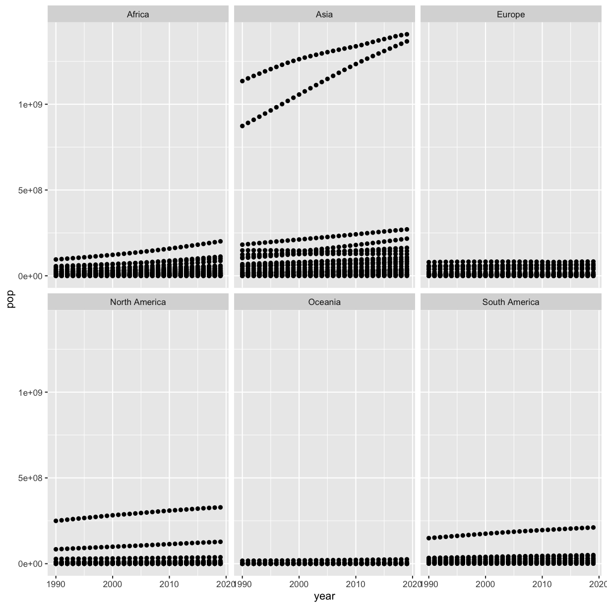
Write some code to figure out which countries these are (even if you already know!).
Solution
smoking %>% filter(pop > 5e8) %>% select(country) %>% distinct()# A tibble: 2 × 1 country <chr> 1 China 2 IndiaHere we used the
distinct()function, which we first saw yesterday. This function is not required to find the answer to this question, but it helps us get the answer a bit more quickly.
Next, plot year vs. population separated into a plot for each continent but excluding the 2 outlier countries. Note that usually you don’t want to exclude certain data points from a plot because it is misleading (see Bonus 2 for an alternative).
Solution
smoking %>%
filter(country != 'China') %>%
filter(country != 'India') %>%
ggplot(aes(x=year,y=pop)) +
geom_point() +
facet_wrap(vars(continent))
Another solution is to use only one filter command and separate the two true/false statements with an ampersand (
&) or comma (,), which means that you want to exclude both China and India:smoking %>% filter(country != 'China' & country != 'India') %>% ggplot(aes(x=year,y=pop)) + geom_point() + facet_wrap(vars(continent))

Bonus 1: Instead of hard-coding the two countries to remove them, remove the two outliers by combining your solutions to the first two questions.
Solution
smoking %>%
filter(pop < 5e8) %>%
ggplot(aes(x=year,y=pop)) +
geom_point() +
facet_wrap(vars(continent))
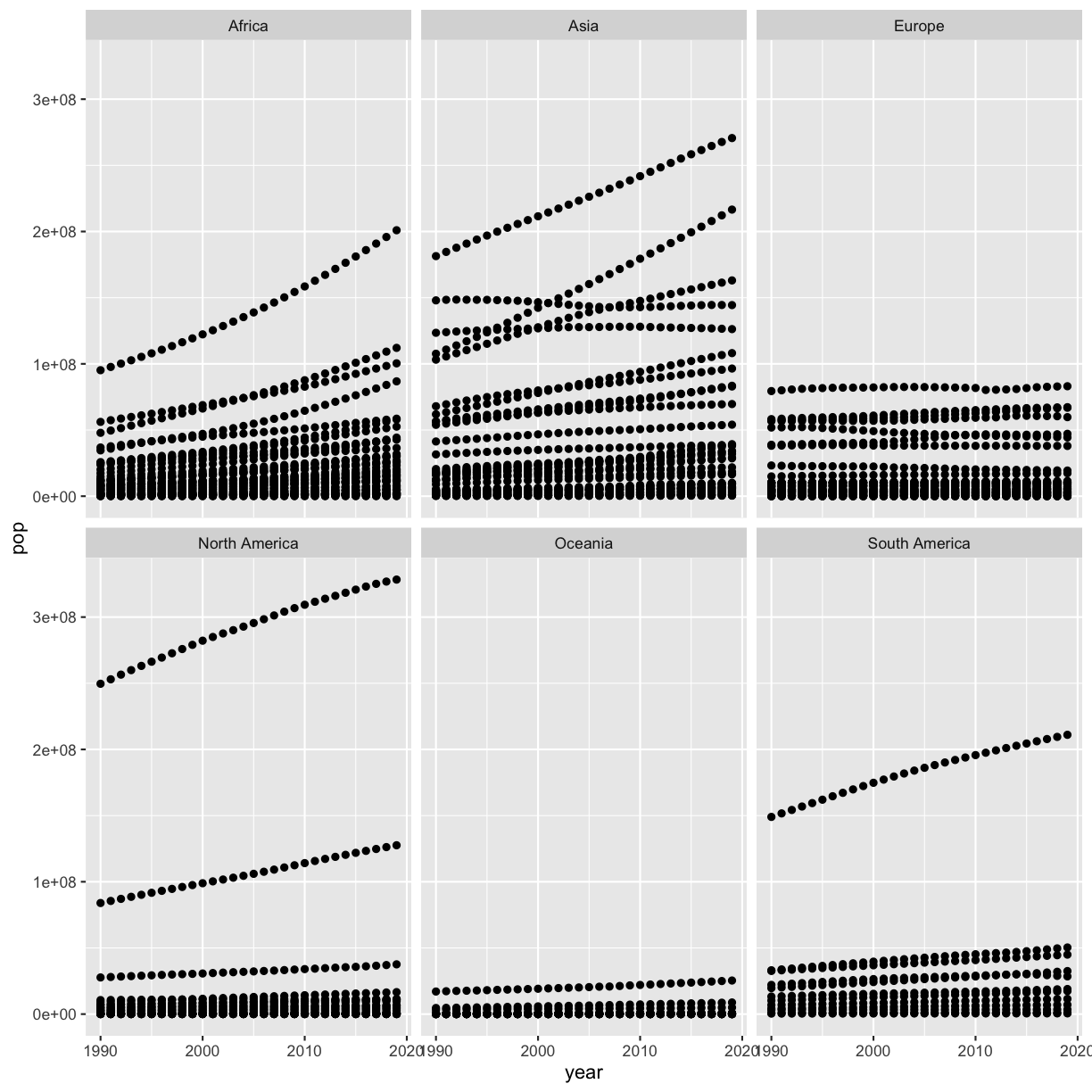
Bonus 2: How can you make the differences between countries more visible on the plot without excluding the two countries you identified above?
Solution
You can scale the y axis using a log10 scale to make the differences more visible:
smoking %>%
ggplot(aes(x=year,y=pop)) +
geom_point() +
scale_y_log10() +
facet_wrap(vars(continent))
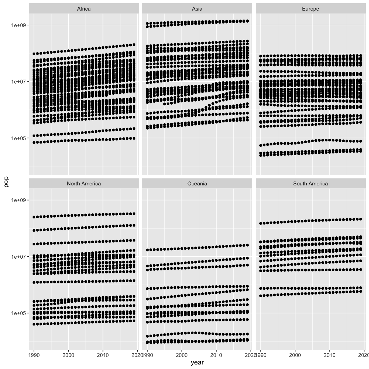
Applying it to your own data
Continue working on your project. Now you can generate some summary statistics as well!
Key Points
Package loading is an important first step in preparing an R environment.
There are many useful functions in the
tidyversepackages that can aid in data analysis.
Writing Reports with R Markdown
Overview
Teaching: 75 min
Exercises: 15 minQuestions
How can I make reproducible reports using R Markdown?
How do I format text using Markdown?
Objectives
To create a report in R Markdown that combines text, code, and figures.
To use Markdown to format our report.
To understand how to use R code chunks to include or hide code, figures, and messages.
To be aware of the various report formats that can be rendered using R Markdown.
Contents
- R for data analysis review
- What is R Markdown and why use it?
- Creating an R Markdown file
- Basic components of R Markdown
- Starting the report
- Customizing the report
- Formatting
- Applying it to your own data
R for data analysis review
Review: Creating summaries
Read in the 1990 smoking dataset and find the mean, median, min, and max population for each continent.
Solution
library(tidyverse)Warning: package 'ggplot2' was built under R version 4.3.3Warning: package 'tibble' was built under R version 4.3.3Warning: package 'purrr' was built under R version 4.3.3Warning: package 'lubridate' was built under R version 4.3.3── Attaching core tidyverse packages ──────────────────────── tidyverse 2.0.0 ── ✔ dplyr 1.1.4 ✔ readr 2.1.5 ✔ forcats 1.0.0 ✔ stringr 1.5.1 ✔ ggplot2 3.5.2 ✔ tibble 3.3.0 ✔ lubridate 1.9.4 ✔ tidyr 1.3.1 ✔ purrr 1.0.4 ── Conflicts ────────────────────────────────────────── tidyverse_conflicts() ── ✖ dplyr::filter() masks stats::filter() ✖ dplyr::lag() masks stats::lag() ℹ Use the conflicted package (<http://conflicted.r-lib.org/>) to force all conflicts to become errorssmoking <- read_csv('data/smoking_cancer_1990.csv')Rows: 191 Columns: 6 ── Column specification ──────────────────────────────────────────────────────── Delimiter: "," chr (2): country, continent dbl (4): year, pop, smoke_pct, lung_cancer_pct ℹ Use `spec()` to retrieve the full column specification for this data. ℹ Specify the column types or set `show_col_types = FALSE` to quiet this message.smoking %>% group_by(continent) %>% summarise(mean_pop = mean(pop), median_pop = median(pop), min_pop = min(pop), max_pop = max(pop))# A tibble: 6 × 5 continent mean_pop median_pop min_pop max_pop <chr> <dbl> <dbl> <dbl> <dbl> 1 Africa 11655968. 6788686. 69507 95212454 2 Asia 75684706. 12446168 223159 1135185000 3 Europe 13056650. 5140939 24124 79433029 4 North America 18257642. 2470946 40260 249623000 5 Oceania 1907505 121440. 8910 17065100 6 South America 24606701. 11752774 405169 149003225
What is R Markdown and why use it?
Recall that our goal is to generate a report on how a country’s smoking rate is related to its lung cancer rate.
Discussion
How do you usually share data analyses with your collaborators?
Solution
Many people share them through a Word or PDF document, a spreadsheet, slides, a graphic, etc.
In R Markdown, you can incorporate ordinary text (ex. experimental methods, analysis and discussion of results) alongside code and figures! (Some people write entire manuscripts in R Markdown.) This is useful for writing reproducible reports and publications, sharing work with collaborators, writing up homework, and keeping a bioinformatics notebook. Because the code is emedded in the document, the tables and figures are reproducible. Anyone can run the code and get the same results. If you find an error or want to add more to the report, you can just re-run the document and you’ll have updated tables and figures! This concept of combining text and code is called “literate programming”. To do this we use R Markdown, which combines Markdown (renders plain text) with R. You can output an html, PDF, or Word document that you can share with others. In fact, this webpage is an example of a rendered R markdown file!
(If you are familiar with Jupyter notebooks in the Python programming environment, R Markdown is R’s equivalent of a Jupyter notebook.)
Creating an R Markdown file
Now that we have a better understanding of what we can use R Markdown files for, let’s start writing a report!
To create an R Markdown file:
- Open RStudio
- Go to File → New File → R Markdown
- Give your document a title, something like “The relationship between smoking and lung cancer rates” (Note: this is not the same as the file name - it’s just a title that will appear at the top of your report)
- Keep the default output format as HTML
- Note: R Markdown files always end in
.Rmd
R Markdown Outputs
The default output for an R Markdown report is HTML, but you can also use R Markdown to output other report formats. For example, you can generate PDF reports using R Markdown, but you must install TeX to do this.
Next, let’s save our R markdown file to the reports directory.
You can do this by clicking the save icon in the top left or using control + s (command + s on a Mac).
Change knit directory
There’s one other thing that we need to do before we get started with our report.
To render our documents into html format, we can “knit” them in R Studio.
Usually, R Markdown renders documents from the directory where the document is saved (the location of the .Rmd file), but we want it to render from the main project directory where our .Rproj file is.
This is because that’s where all of our relative paths are from and it’s good practice to have all of your relative paths from the main project directory.
To change this default, click on the down arrow next to the “Knit” button at the top left of R Studio, go to “Knit Directory” and click “Project Directory”.
Now it will assume all of your relative paths for reading and writing files are from the un-report directory, rather than the reports directory.
Now that we have that set up, let’s start on the report!
Add code
We’re going to use the code you generated yesterday to plot smoking rates vs. lung cancer rates to include in the report. Recall that we needed a couple R packages to generate these plots. We can create a new code chunk to load the needed packages. You could also include this in the previous setup chunk, it’s up to your personal preference. To create a new code chunk, you have several options: type it out yourself, click the button with the green c and + in the top right, next to Run, or use the keyboard shortcut Ctrl + Alt + i.
```{r packages}
library(tidyverse)
```
Now, in a real report this is when we would type out the background and purpose of our analysis to provide context to our readers. However, since writing is not a focus of this workshop we will avoid lengthy prose and stick to short descriptions. You can copy the following text into your own report below the package code chunk.
This report was prepared to analyze the relationship between a country's lung cancer rate, smoking rate, and air pollution. Our goal is to determine to what degree the percent of people who smoke and the amount of air pollution per capita may be related to its lung cancer rate. We hypothesize that lung cancer rates increase with both percent of people who smoke and the amount of air pollution per capita.
Now, since we want to show our results comparing smoking rate and lung cancer rate by country, we need to read in this data so we can generate our plot. We will add another code chunk to prepare the data.
```{r data}
smoking <- read_csv("data/smoking_cancer.csv")
```
Plot
Now that we have the data, we need to produce the plot. Let’s create it using the most recent year in our dataset:
```{r smoking_cancer}
smoking %>%
  filter(year == max(year)) %>%
  ggplot() +
  aes(x = smoke_pct, y = lung_cancer_pct, color=continent, size=pop/1000000) +
  geom_point() +
  labs(x = "Percent of people who smoke", y = "Percent of people with lung cancer",
       title= "Are lung cancer rates associated with smoking rates?", size="Population (in millions)")
```
Table
Let’s say we also want to include a table in our report that summarizes the the minimum, median, and maximum smoker percent.
```{r}
smoking %>%
  summarize(min_smoke = min(smoke_pct),
            median_smoke = median(smoke_pct),
            max_smoke = max(smoke_pct))
```
Knitting
Now we can knit our document to see how our report looks! Use the knit button in the top left of the screen.
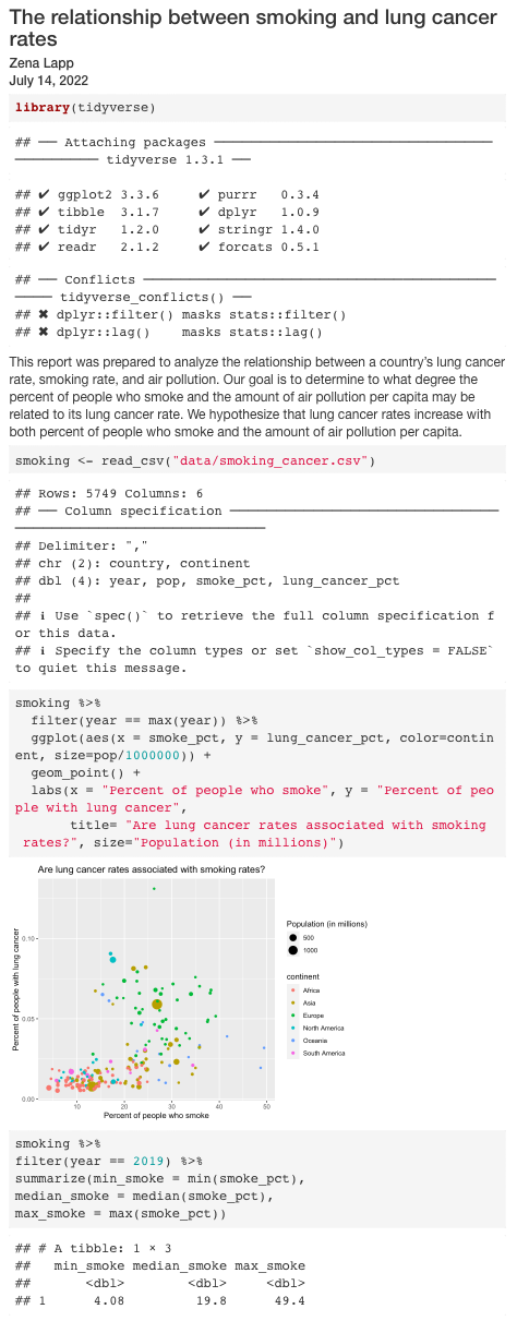
Amazing! We’ve created a report!
It’s looking pretty good, but there seem to be a few extra bits that we might not need in the report. For example, what if we want to make a report that doesn’t print out all of the messages from the tidyverse? Or a report that doesn’t show the code? And the table is a bit ugly. Let’s make things a bit prettier.
Customizing the report
Table format
We can make the table prettier using the R function kable(). We can give the kable() function a tibble and it will format it to a nice looking table in the report. The kable() function comes from the knitr packages, so what do we have to do before using the function? We have to load the knitr library.
# load library
library(knitr)

# print kable
smoking %>%
   summarize(min_smoke = min(smoke_pct),
             median_smoke = median(smoke_pct),
             max_smoke = max(smoke_pct)) %>%
  kable()
| min_smoke| median_smoke| max_smoke|
|---------:|------------:|---------:|
|  3.118639|     24.36522|  46.91547|
Messages
How do we get rid of the tidyverse messages? One way to do this is by saying include = FALSE in the curly brackets for that code chunk:
```{r packages, include=FALSE}
library(tidyverse)
```
This will get rid of the code and the corresponding messages. But what if we want to include the code so that people know we loaded the tidyverse? In this case, we can say message=FALSE inside the curly brackets:
```{r packages, message=FALSE}
library(tidyverse)
```
Code
We can also see the code that was used to generate the plot. Depending on the purpose and audience for your report, you may or may not want to include the code. If you don’t want the code to appear, how can you prevent it?
Code chunk options
Which of the following would lead to a report with no code chunks? For the ones that would not work, what would happen instead?
- Add
echo = FALSEinside the curly brackets of the plotting code chunk.- Add
include = FALSEinside the curly brackets of the plotting code chunk.- Add
echo = FALSEinside the curly brackets of the setup code chunk.- Change
echo = TRUEtoecho = FALSEin theknitr::opts_chunk$set()function in the first code chunk.Solution
- This would only remove the code for the plotting code chunk, but not the packages code chunk.
- This would remove the code but also the plot from the report.
- This would not change anything because that code chunk is already excluded because
include = FALSE.- This would remove all code from the output file (what we want).
Add to our report: association between air pollution and lung cancer
We have a pretty nice looking report, but we still haven’t included anything about the association between lung cancer and air pollution per capita. Let’s add a section to our markdown document in the following steps:
- Make a new header and write a 1-2 sentence description of what you will be plotting.
- Create a new code chunk
- Make a plot with air pollution per capita on the x axis and lung cancer on the y axis
- Make a table with summary statistics including the minimum, median, and maximum air pollution values.
- BONUS: Merge the table we created earlier with the table you created here with rows for smoking and air pollution, and a column for each of the summary statistics.
Solution
One option to create a code chunk is to type it out. You can also see other options above. Then you have to read in the data and create the plot and table:
smoking_pollution <- read_csv('data/smoking_pollution.csv')Rows: 191 Columns: 7 ── Column specification ──────────────────────────────────────────────────────── Delimiter: "," chr (2): country, continent dbl (5): year, pop, smoke_pct, lung_cancer_pct, pollution ℹ Use `spec()` to retrieve the full column specification for this data. ℹ Specify the column types or set `show_col_types = FALSE` to quiet this message.smoking_pollution %>% ggplot(aes(x = pollution/pop, y = lung_cancer_pct)) + geom_point() + labs(x = "Ambient pollution (micrograms/cubic meter) per capita", y = "Percent of people with lung cancer", title = "Are lung cancer rates associated with pollution per capita?")
smoking_pollution %>%
 summarize(min_pol = min(pollution),
            median_smoke = median(pollution),
            max_smoke = max(pollution))
# A tibble: 1 × 3 min_pol median_smoke max_smoke <dbl> <dbl> <dbl> 1 4.69 24.5 78.2Bonus: you can use
pivot_longer()andgroup_by()followed bysummarize():smoking_pollution %>% pivot_longer(c(smoke_pct, pollution)) %>% group_by(name) %>% summarize(min = min(value), median = median(value), max = max(value))# A tibble: 2 × 4 name min median max <chr> <dbl> <dbl> <dbl> 1 pollution 4.69 24.5 78.2 2 smoke_pct 3.12 24.4 46.9Notice that we used
c()to providepivot_longer()with the two column names that we wanted to pivot.c()stands for “combine”; this function combines the two values into what we call a vector.
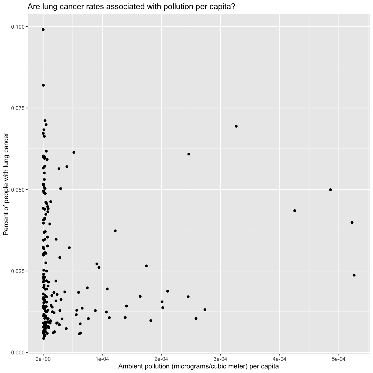
Bonus: Dynamically updating text using mini R chunks
Sometimes, you want to describe your data or results (like our plot) to the audience in text but the data and results may still change as you work things out. R Markdown offers an easy way to do this dynamically, so that the text updates as your data or results change!
Say we want to get the number of countries present in our dataset. Previously, we learned about the
distinct()function that returns distinct values. There’s a very similar function calledn_distinct()that returns instead the number of distinct values:n_countries <- smoking %>% select(country) %>% n_distinct()Now, all we need to do is reference the values we just computed to describe our plot. To do this, we enclose each value in one set of backticks (
`r some_R_variable_name `), while therpart once again indicates that it’s a chunk of R code. When we knit our report, R will automatically fill in the values we just created in the above code chunk. Note that R will automatically update these values every time our data might change (if we were to decide to drop or add countries to this analysis, for example).There are `r n_countries ` countries in our dataset.Try knitting the document and see what happens!
Key Points
R Markdown is a useful way to create a report that integrates text, code, and figures.
Options such as
includeandechodetermine what parts of an R code chunk are included in the R Markdown report.R Markdown can render HTML, PDF, and Microsoft Word outputs.
Conclusion
Overview
Teaching: 15 min
Exercises: minQuestions
What do I do after the workshop to apply what I learned and keep learning more?
How do I deal with coding errors (i.e. debug)?
Objectives
Learn how to get help with code via the Internet and reaching out to others.
Contents
Workshop summary & moving forward
Congratulations on completing the workshop! You learned some basic procedures for importing, managing, visualizing and reporting your data. The absolute best way to continue improving your skills is to use R in your own work, e.g. to automate a task, to analyze data, or to create reports.
Brainstorm session: how to use R as much as possible
How can you use R in your work to be able to keep improving your skills?
Solution:
Is there a task you can automate, data you wish to analyze or visualize, or reports that you need to make?
As you continue on your coding journey, you will want to learn new data processing and analysis techniques.
As we complete the course, we want to share with you some tips and tricks that have helped us on our own programming journeys.
Learning more and getting help
The Internet
The Internet is your best friend.
If you get stuck, use your favorite search engine to look for an answer to your question. An example is “how to import an excel spreadsheet into R.” Typically, you will find step-by-step online documentation that you can adapt for your own purposes.
If you want to learn something new, use your favorite search engine to look for tutorials and other resources related to the topic.
Additional coding topics
There are some coding concepts that we did not have time to cover in this workshop, but are important to learn as you continue on your journey and begin to perform more sophisticated data analysis projects. We’ve provided some links below, but feel free to search for other explanations and tutorials as well.
Here is a nice tutorial on conditionals, loops, and functions all together.
Domain-specific analyses
We encourage you to investigate domain-specific packages and software that will help you perform specific tasks related to your own research. You can find these packages through:
- Other people in the field.
- Internet searches with keywords related to the topic of interest, including R (the programming language you’re interested in using; e.g. “find pairwise distances for DNA sequences in R”).
Reach out to others
We want to be a resource for you after the workshop ends, and we also want you all to be a resource for each other.
You can email us whenever you want with questions! If it’s a quick thing, we can figure out over email, otherwise we can set up a time to chat.
We are always monitoring the following address: discovr.workshop@gmail.com
Here are our personal emails:
- Christine: christine.markwalter@duke.edu
- Emmah: kimachasnr@gmail.com
What to include when asking for help
- A brief summary of what you are trying to accomplish (your ultimate goal, distilled into one specific question).
- Brief description of what you’ve tried so far.
- Description of the problem you’re having - the exact code you used, the expected output, the actual error/output.
- A minimal, reproducible example. Include the code and data (or made-up data) you need to reproduce the error.
Code club
For additional consistent support, we will be hosting a monthly virtual code club where we will discuss different coding topics and troubleshoot issues you may be having with your own data. Please let us know if you would like to participate.
Key Points
Using R regularly is the best way to improve your skills.
When it comes to trying to figure out how to code something, and debugging, Internet searching is your best friend.
Don’t be afraid to reach out to others and ask for help.