Writing Reports with R Markdown

Overview

Teaching: 75 min
Exercises: 15 min

Questions

How can I make reproducible reports using R Markdown?

How do I format text using Markdown?

Objectives

To create a report in R Markdown that combines text, code, and figures.

To use Markdown to format our report.

To understand how to use R code chunks to include or hide code, figures, and messages.

To be aware of the various report formats that can be rendered using R Markdown.

R for data analysis review
What is R Markdown and why use it?
Creating an R Markdown file
Basic components of R Markdown
- Header
- Code chunks
- Text
Starting the report
Customizing the report
- Table format
- Messages
- Code
- Bonus
Formatting
- Headers
- Lists
Applying it to your own data

R for data analysis review

Review: Creating summaries

Read in the 1990 smoking dataset and find the mean, median, min, and max population for each continent.

Solution

library(tidyverse)

── Attaching core tidyverse packages ──────────────────────── tidyverse 2.0.0 ──
✔ dplyr     1.1.2     ✔ readr     2.1.4
✔ forcats   1.0.0     ✔ stringr   1.5.0
✔ ggplot2   3.4.2     ✔ tibble    3.2.1
✔ lubridate 1.9.2     ✔ tidyr     1.3.0
✔ purrr     1.0.1     
── Conflicts ────────────────────────────────────────── tidyverse_conflicts() ──
✖ dplyr::filter() masks stats::filter()
✖ dplyr::lag()    masks stats::lag()
ℹ Use the conflicted package (<http://conflicted.r-lib.org/>) to force all conflicts to become errors

smoking <- read_csv('data/smoking_cancer_1990.csv')

Rows: 191 Columns: 6
── Column specification ────────────────────────────────────────────────────────
Delimiter: ","
chr (2): country, continent
dbl (4): year, pop, smoke_pct, lung_cancer_pct

ℹ Use `spec()` to retrieve the full column specification for this data.
ℹ Specify the column types or set `show_col_types = FALSE` to quiet this message.

smoking %>% 
  group_by(continent) %>% 
  summarise(mean_pop = mean(pop),
            median_pop = median(pop),
            min_pop = min(pop),
            max_pop = max(pop))

# A tibble: 6 × 5
  continent      mean_pop median_pop min_pop    max_pop
  <chr>             <dbl>      <dbl>   <dbl>      <dbl>
1 Africa        11655968.   6788686.   69507   95212454
2 Asia          75684706.  12446168   223159 1135185000
3 Europe        13056650.   5140939    24124   79433029
4 North America 18257642.   2470946    40260  249623000
5 Oceania        1907505     121440.    8910   17065100
6 South America 24606701.  11752774   405169  149003225

What is R Markdown and why use it?

Back to top

Recall that our goal is to generate a report on how a country’s smoking rate is related to its lung cancer rate.

Discussion

How do you usually share data analyses with your collaborators?

Solution

Many people share them through a Word or PDF document, a spreadsheet, slides, a graphic, etc.

In R Markdown, you can incorporate ordinary text (ex. experimental methods, analysis and discussion of results) alongside code and figures! (Some people write entire manuscripts in R Markdown.) This is useful for writing reproducible reports and publications, sharing work with collaborators, writing up homework, and keeping a bioinformatics notebook. Because the code is emedded in the document, the tables and figures are reproducible. Anyone can run the code and get the same results. If you find an error or want to add more to the report, you can just re-run the document and you’ll have updated tables and figures! This concept of combining text and code is called “literate programming”. To do this we use R Markdown, which combines Markdown (renders plain text) with R. You can output an html, PDF, or Word document that you can share with others. In fact, this webpage is an example of a rendered R markdown file!

(If you are familiar with Jupyter notebooks in the Python programming environment, R Markdown is R’s equivalent of a Jupyter notebook.)

Creating an R Markdown file

Back to top

Now that we have a better understanding of what we can use R Markdown files for, let’s start writing a report!

To create an R Markdown file:

Open RStudio
Go to File → New File → R Markdown
Give your document a title, something like “The relationship between smoking and lung cancer rates” (Note: this is not the same as the file name - it’s just a title that will appear at the top of your report)
Keep the default output format as HTML
Note: R Markdown files always end in .Rmd

R Markdown Outputs

The default output for an R Markdown report is HTML, but you can also use R Markdown to output other report formats. For example, you can generate PDF reports using R Markdown, but you must install TeX to do this.

Basic components of R Markdown

Back to top

The first part of every R markdown file is a header at the top of the file between the lines of ---. This contains instructions for R to specify the type of document to be created and options to choose (ex., title, author, date). These are in the form of key-value pairs (key: value; YAML).

Here’s an example:

---
title: 'The relationship between smoking and lung cancer rates'
author: "Zena Lapp"
date: "July 14, 2022"
output: html_document
---

Code chunks

Back to top

The next section is a code chunk, or embedded R code, that sets up options for all code chunks. Here is the default when you create a new R Markdown file:

```{r setup, include=FALSE}
knitr::opts_chunk$set(echo = TRUE)
```

All code chunks have this format:

```{r}
# Your code here
```

All of the code is enclosed in 3 back ticks (), and the {r} part indicates that it’s a chunk of R code.

You can also include other information within the curly brackets to indicate different information about that code chunk. For instance, the first code block is named “setup”, and include=FALSE prevents code and results from showing up in the output file.

Inside the code chunk, you can put any R code that you want to run, and you can have as many code chunks as you want in your file.

As we mentioned above, in the first code chunk you set options for the entire file. echo = TRUE means that you want your code to be shown in the output file. If you change this to echo = FALSE, then the code will be hidden and only the output of the code chunks will be seen in the output file. There are also many other options that you can change, but we won’t go into those details in this workshop.

Text

Back to top

Finally, you can include text in your R Markdown file. This is any text or explanation you want to include, and it’s formatted with Markdown. We’ll learn more about Markdown formatting soon!

Starting the report

Back to top

Let’s return to the new R Markdown file you created and delete everything below the setup code chunk. (That stuff is just examples and reminders of how to use R Markdown.)

Next, let’s save our R markdown file to the reports directory. You can do this by clicking the save icon in the top left or using control + s (command + s on a Mac).

Change knit directory

There’s one other thing that we need to do before we get started with our report. To render our documents into html format, we can “knit” them in R Studio. Usually, R Markdown renders documents from the directory where the document is saved (the location of the .Rmd file), but we want it to render from the main project directory where our .Rproj file is. This is because that’s where all of our relative paths are from and it’s good practice to have all of your relative paths from the main project directory. To change this default, click on the down arrow next to the “Knit” button at the top left of R Studio, go to “Knit Directory” and click “Project Directory”. Now it will assume all of your relative paths for reading and writing files are from the un-report directory, rather than the reports directory.

Now that we have that set up, let’s start on the report!

Add code

We’re going to use the code you generated yesterday to plot smoking rates vs. lung cancer rates to include in the report. Recall that we needed a couple R packages to generate these plots. We can create a new code chunk to load the needed packages. You could also include this in the previous setup chunk, it’s up to your personal preference. To create a new code chunk, you have several options: type it out yourself, click the button with the green c and + in the top right, next to Run, or use the keyboard shortcut Ctrl + Alt + i.

```{r packages}
library(tidyverse)
```

Now, in a real report this is when we would type out the background and purpose of our analysis to provide context to our readers. However, since writing is not a focus of this workshop we will avoid lengthy prose and stick to short descriptions. You can copy the following text into your own report below the package code chunk.

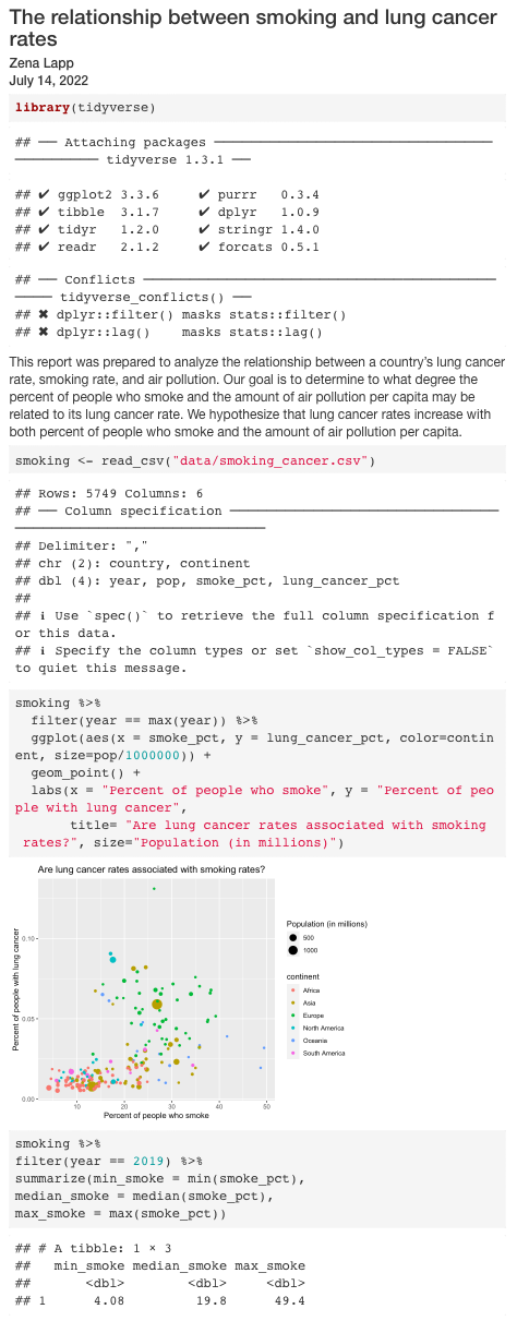
This report was prepared to analyze the relationship between a country's lung cancer rate, smoking rate, and air pollution. Our goal is to determine to what degree the percent of people who smoke and the amount of air pollution per capita may be related to its lung cancer rate. We hypothesize that lung cancer rates increase with both percent of people who smoke and the amount of air pollution per capita.

Now, since we want to show our results comparing smoking rate and lung cancer rate by country, we need to read in this data so we can generate our plot. We will add another code chunk to prepare the data.

```{r data}
smoking <- read_csv("data/smoking_cancer.csv")
```

Plot

Now that we have the data, we need to produce the plot. Let’s create it using the most recent year in our dataset:

```{r smoking_cancer}
smoking %>%
  filter(year == max(year)) %>% 
  ggplot() + 
  aes(x = smoke_pct, y = lung_cancer_pct, color=continent, size=pop/1000000) +
  geom_point() +
  labs(x = "Percent of people who smoke", y = "Percent of people with lung cancer",
       title= "Are lung cancer rates associated with smoking rates?", size="Population (in millions)")
```

Table

Let’s say we also want to include a table in our report that summarizes the number of countries, the minimum smoker percent, and the maximum smoker percent.

```{r}
smoking %>% 
  summarize(min_smoke = min(smoke_pct),
            median_smoke = median(smoke_pct),
            max_smoke = max(smoke_pct))
```

Knitting

Now we can knit our document to see how our report looks! Use the knit button in the top left of the screen.

Amazing! We’ve created a report!

It’s looking pretty good, but there seem to be a few extra bits that we might not need in the report. For example, what if we want to make a report that doesn’t print out all of the messages from the tidyverse? Or a report that doesn’t show the code? And the table is a bit ugly. Let’s make things a bit prettier.

Customizing the report

Table format

We can make the table prettier using the R function kable(). We can give the kable() function a tibble and it will format it to a nice looking table in the report. The kable() function comes from the knitr packages, so what do we have to do before using the function? We have to load the knitr library.

# load library
library(knitr)

# print kable
smoking %>% 
   summarize(min_smoke = min(smoke_pct),
             median_smoke = median(smoke_pct),
             max_smoke = max(smoke_pct)) %>%
  kable()

min_smoke	median_smoke	max_smoke
3.118639	24.36522	46.91547

Messages

How do we get rid of the tidyverse messages? One way to do this is by saying include = FALSE in the curly brackets for that code chunk:

```{r packages, include=FALSE}
library(tidyverse)
```

This will get rid of the code and the corresponding messages. But what if we want to include the code so that people know we loaded the tidyverse? In this case, we can say message=FALSE inside the curly brackets:

```{r packages, message=FALSE}
library(tidyverse)
```

Code

We can also see the code that was used to generate the plot. Depending on the purpose and audience for your report, you may or may not want to include the code. If you don’t want the code to appear, how can you prevent it?

Code chunk options

Which of the following would lead to a report with no code chunks? For the ones that would not work, what would happen instead?

Add echo = FALSE inside the curly brackets of the plotting code chunk.

Add include = FALSE inside the curly brackets of the plotting code chunk.

Add echo = FALSE inside the curly brackets of the setup code chunk.

Change echo = TRUE to echo = FALSE in the knitr::opts_chunk$set() function in the first code chunk.

Solution

This would only remove the code for the plotting code chunk, but not the packages code chunk.

This would remove the code but also the plot from the report.

This would not change anything because that code chunk is already excluded because include = FALSE.

This would remove all code from the output file (what we want).

Formatting

Back to top

We now know how to create a report with R Markdown. Maybe we also want to format the report a little bit to structure our thought process in a useful way (e.g., sections) and make it visually appealing? Markdown is like a simple programming language when it comes to syntax. Let’s try to figure out some syntax together. Suppose we wanted to create sections in our report.

Headers

To create different sections by using headers and sub-headers, you can use the # (pound/hash) sign. Our main headers have one # (e.g. # Main Header Here) and to create subheaders we add additinal #s (e.g. ## First subheader and ### Second subheader)

Lists

To create a bulleted list in R Markdown, you can use the - (dash) or the * (asterisk). Create a bulleted list with three items:

* The name of your currently favorite programming language 
* The name of a function you have so far found most useful 
* One thing you want to learn next on your programming journey

Bold and italics

Use the Internet or the R Markdown reference guide to figure out how to: 1) bold the text of the first bullet point, 2) italicize the text of the second bullet point, 3) bold and italicize the text of the third bullet point.

Solution

Italics can be generated by enclosing the text in _ (single underscores) or * (single asterisks), and bold in __ (double underscores) or ** (double asterisks). To use both, use three instead underscores (___) or asterisks (***) instead.

Okay, now how do you think we’d turn our bulleted list into a numbered list?

You can change the bullets to numbers with dots after them:

The name of your currently favorite programming language 
The name of a function you have so far found most useful 
One thing you want to learn next on your programming journey

Or, even better, you can just make them all 1. and markdown will be smart enough to number them in order. This is super useful if you end up wanting to add in an item in the middle of the list:

The name of your currently favorite programming language 
The name of a function you have so far found most useful 
One thing you want to learn next on your programming journey

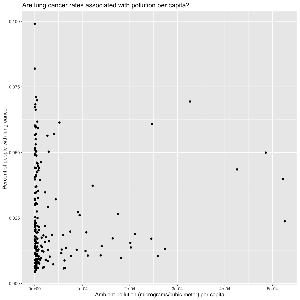
Add to our report: association between air pollution and lung cancer

We have a pretty nice looking report, but we still haven’t included anything about the association between lung cancer and air pollution per capita. Let’s add a section to our markdown document in the following steps:

Make a new header and write a 1-2 sentence description of what you will be plotting.

Create a new code chunk

Make a plot with air pollution per capita on the x axis and lung cancer on the y axis

Make a table with summary statistics including the minimum, median, and maximum air pollution values.

BONUS: Merge the table we created earlier with the table you created here with rows for smoking and air pollution, and a column for each of the summary statistics.
Solution

One option to create a code chunk is to type it out. You can also see other options above. Then you have to read in the data and create the plot and table:
smoking_pollution <- read_csv('data/smoking_pollution.csv')
Rows: 191 Columns: 7
── Column specification ────────────────────────────────────────────────────────
Delimiter: ","
chr (2): country, continent
dbl (5): year, pop, smoke_pct, lung_cancer_pct, pollution

ℹ Use `spec()` to retrieve the full column specification for this data.
ℹ Specify the column types or set `show_col_types = FALSE` to quiet this message.
smoking_pollution %>%
  ggplot(aes(x = pollution/pop, y = lung_cancer_pct)) + 
  geom_point() +
  labs(x = "Ambient pollution (micrograms/cubic meter) per capita", y = "Percent of people with lung cancer",
       title = "Are lung cancer rates associated with pollution per capita?")
smoking_pollution %>% 
 summarize(min_pol = min(pollution),
            median_smoke = median(pollution),
            max_smoke = max(pollution))
# A tibble: 1 × 3
  min_pol median_smoke max_smoke
    <dbl>        <dbl>     <dbl>
1    4.69         24.5      78.2
Bonus: you can use pivot_longer() and group_by() followed by summarize():
smoking_pollution %>%
  pivot_longer(c(smoke_pct, pollution)) %>% 
  group_by(name) %>% 
  summarize(min = min(value),
            median = median(value),
            max = max(value))
# A tibble: 2 × 4
  name        min median   max
  <chr>     <dbl>  <dbl> <dbl>
1 pollution  4.69   24.5  78.2
2 smoke_pct  3.12   24.4  46.9
Notice that we used c() to provide pivot_longer() with the two column names that we wanted to pivot. c() stands for “combine”; this function combines the two values into what we call a vector.

Bonus: Dynamically updating text using mini R chunks

Sometimes, you want to describe your data or results (like our plot) to the audience in text but the data and results may still change as you work things out. R Markdown offers an easy way to do this dynamically, so that the text updates as your data or results change!

Say we want to get the number of countries present in our dataset. Previously, we learned about the distinct() function that returns distinct values. There’s a very similar function called n_distinct() that returns instead the number of distinct values:
n_countries <- smoking %>%
  select(country) %>%
  n_distinct()
Now, all we need to do is reference the values we just computed to describe our plot. To do this, we enclose each value in one set of backticks (`r some_R_variable_name `), while the r part once again indicates that it’s a chunk of R code. When we knit our report, R will automatically fill in the values we just created in the above code chunk. Note that R will automatically update these values every time our data might change (if we were to decide to drop or add countries to this analysis, for example).
There are `r n_countries ` countries in our dataset. 
Try knitting the document and see what happens!

Applying it to your own data

Now it’s time to merge all of your analyses with your own data together into a report. Fill out the worksheet to outline your report and then start making it!

Key Points

R Markdown is a useful way to create a report that integrates text, code, and figures.

Options such as include and echo determine what parts of an R code chunk are included in the R Markdown report.

R Markdown can render HTML, PDF, and Microsoft Word outputs.

previous episode

DiscovR Workshop Curriculum

next episode

Writing Reports with R Markdown

Overview

Contents

R for data analysis review

Review: Creating summaries

Solution

What is R Markdown and why use it?

Discussion

Solution

Creating an R Markdown file

R Markdown Outputs

Basic components of R Markdown

Header

Code chunks

Text

Starting the report

Change knit directory

Add code

Plot

Table

Knitting

Customizing the report

Table format

Messages

Code

Code chunk options

Solution

Formatting

Headers

Lists

Bold and italics

Solution

Add to our report: association between air pollution and lung cancer

Solution

Bonus: Dynamically updating text using mini R chunks

Applying it to your own data

Key Points

previous episode

next episode