R for Data Cleaning

Overview

Teaching: 105 min
Exercises: 30 min

Questions

How can I clean my data in R?

How can I combine two datasets from different sources?

How can R help make my research more reproducible?

Objectives

To become familiar with the functions of the dplyr and tidyr packages.

To be able to clean and prepare datasets for analysis.

To be able to combine two different data sources using joins.

Cleaning up data
Day 1 review
Overview of the lesson
Narrow down rows with filter()
Subset columns using select()
Checking for missing values
Checking for duplicate rows
Grouping and counting rows using group_by()
Make new variables with mutate()
Joining dataframes

Cleaning up data

Back to top

Researchers are often pulling data from several sources, and the process of making data compatible with one another and prepared for analysis can be a large undertaking. Luckily, there are many functions that allow us to do this in R. Yesterday, we worked with the Global Burden of Disease (GBD 2019) dataset, which contains population, smoking rates, and lung cancer rates by year (we only used 1990). Today, we will practice cleaning and preparing a second dataset containing ambient pollution data by location and year, also sourced from the GBD 2019.

It’s always good to go into data cleaning with a clear goal in mind. Here, we’d like to prepare the ambient pollution data to be compatible with our lung cancer data so we can directly compare lung cancer rates to ambient pollution levels (we will do this tomorrow). To make this work, we’d like a dataframe that contains columns with the country name, year, and median ambient pollution levels (in micrograms per cubic meter). We will make this comparison for the first year in these datasets, 1990.

Let’s start with reviewing how to read in the data.

Day 1 review

Opening your Rproject in RStudio.

First, navigate to the un-reports directory however you’d like and open un-report.Rproj. This should open the un-report R project in RStudio. You can check this by seeing if the Files in the bottom right of RStudio are the ones in your un-report directory.

Creating a new R script.

Then create a new R Script file for our work. Open RStudio. Choose “File” > “New File” > “RScript”. Save this file as un_data_cleaning.R.

Loading your data.

Now, let’s import the pollution dataset into our fresh new R session. It’s not clean yet, so let’s call it ambient_pollution_dirty

ambient_pollution_dirty <- read_csv("data/ambient_pollution.csv")

Error in read_csv("data/ambient_pollution.csv"): could not find function "read_csv"

Exercise: What error do you get and why?

Fix the code so you don’t get an error and read in the dataset. Hint: Packages…
Solution

If we look in the console now, we’ll see we’ve received an error message saying that R “could not find the function read_csv()”. What this means is that R cannot find the function we are trying to call. The reason for this usually is that we are trying to run a function from a package that we have not yet loaded. This is a very common error message that you will probably see a lot when using R. It’s important to remember that you will need to load any packages you want to use into R each time you start a new session. The read_csv function comes from the readr package which is included in the tidyverse package so we will just load the tidyverse package and run the import code again:
library(tidyverse)
── Attaching core tidyverse packages ──────────────────────── tidyverse 2.0.0 ──
✔ dplyr     1.1.2     ✔ readr     2.1.4
✔ forcats   1.0.0     ✔ stringr   1.5.0
✔ ggplot2   3.4.2     ✔ tibble    3.2.1
✔ lubridate 1.9.2     ✔ tidyr     1.3.0
✔ purrr     1.0.1     
── Conflicts ────────────────────────────────────────── tidyverse_conflicts() ──
✖ dplyr::filter() masks stats::filter()
✖ dplyr::lag()    masks stats::lag()
ℹ Use the conflicted package (<http://conflicted.r-lib.org/>) to force all conflicts to become errors
ambient_pollution_dirty <- read_csv("data/ambient_pollution.csv")
Rows: 9660 Columns: 3
── Column specification ────────────────────────────────────────────────────────
Delimiter: ","
chr (1): location_name
dbl (2): year_id, median

ℹ Use `spec()` to retrieve the full column specification for this data.
ℹ Specify the column types or set `show_col_types = FALSE` to quiet this message.
As we saw yesterday, the output in your console shows that by doing this, we attach several useful packages for data wrangling, including readr and dplyr. Check out these packages and their documentation at tidyverse.org.

Reminder: Many of these packages, including dplyr, come with “Cheatsheets” found under the Help RStudio menu tab.

Now, let’s take a look at what this data object contains:

ambient_pollution_dirty

# A tibble: 9,660 × 3
   location_name year_id median
   <chr>           <dbl>  <dbl>
Global           1990   40.0
Global           1995   38.9
Global           2000   40.6
Global           2005   40.6
Global           2010   42.7
Global           2011   44.4
Global           2012   46.1
Global           2013   47.1
Global           2014   47.3
Global           2015   46.1
# ℹ 9,650 more rows

It looks like our data object has three columns: location_name, year_id, and median. Median here is the median ambient pollution in micrograms per cubic meter. Scroll through the data object to get an idea of what’s there.

Plotting review: median pollution levels

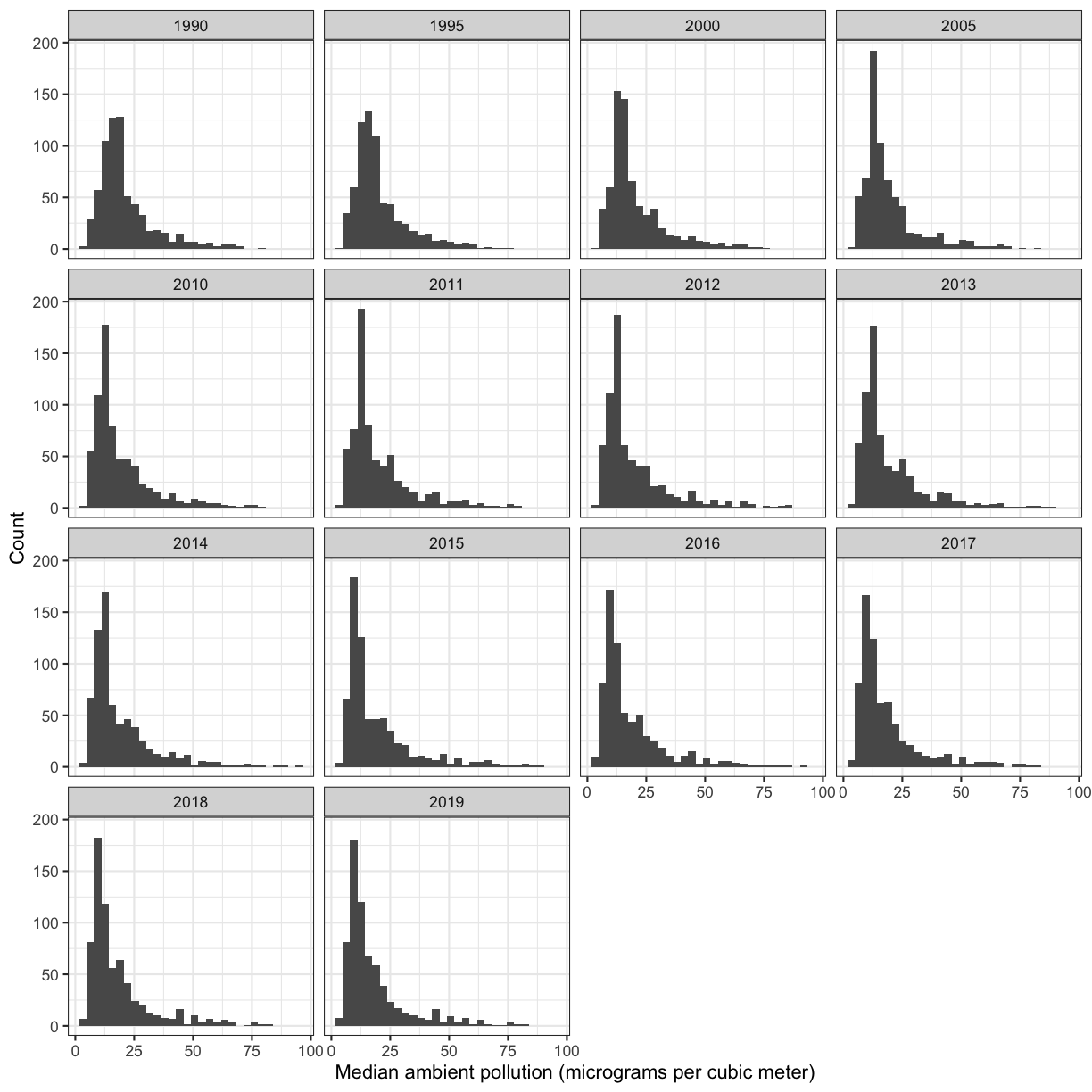
Let’s refresh out plotting skills. Make a histogram of pollution levels in the ambient_pollution_dirty data object. Feel free to look back at the content from yesterday if you want!

Bonus 1: Facet by year_id to look at histograms of ambient pollution levels for each year in the dataset.

Bonus 2: Make the plot prettier by changing the axis labels, theme, and anything else you want.
Solution
ggplot(ambient_pollution_dirty, aes(x = median)) +
  geom_histogram()
`stat_bin()` using `bins = 30`. Pick better value with `binwidth`.
Bonus 1:
ggplot(ambient_pollution_dirty) +
  aes(x = median) +
  geom_histogram() +
  facet_wrap(~year_id)
`stat_bin()` using `bins = 30`. Pick better value with `binwidth`.
Bonus 2 example:
ggplot(ambient_pollution_dirty, aes(x = median)) +
  geom_histogram() +
  facet_wrap(~year_id) +
  labs(x = 'Median ambient pollution (micrograms per cubic meter)', y = 'Count') +
  theme_bw()
`stat_bin()` using `bins = 30`. Pick better value with `binwidth`.

Overview of the lesson

Back to top

Great, now that we’ve read in the data and practiced plotting, we can start to think about cleaning the data. Remember that our goal is to prepare the ambient pollution data to be compatible with our lung cancer rates so we can directly compare lung cancer rates to ambient pollution levels (we will do this tomorrow). To make this work, we’d like a dataframe that contains columns with the country name, year, and median ambient pollution levels (in micrograms per cubic meter). We will make this comparison for the first year in these datasets, 1990.

What data cleaning do we have to do?

Look back at the three columns in our data object: location_name, year_id, and median. What might we need to take care of in order to merge these data with our lung cancer rates dataset?

Solution

It looks like the location_name column contains values other than countries, and our year_id column has many years, and we are only interested in 1990 for now.

Narrow down rows with `filter()`

Back to top

Let’s start by narrowing the dataset to only the year 1990. To do this, we will use the filter() function. Here’s what that looks like:

filter(ambient_pollution_dirty, year_id = 1990)

Error in `filter()`:
! We detected a named input.
ℹ This usually means that you've used `=` instead of `==`.
ℹ Did you mean `year_id == 1990`?

Oops! We got an error, but don’t panic. Error messages are often pretty useful. In this case, it says that that we used = instead of ==. That’s because we use = (single equals) when naming arguments that you are passing to functions. So here R thinks we’re trying to assign 1990 to year, kind of like we do when we’re telling ggplot what we want our aesthetics to be. What we really want to do is find all of the years that are equal to 1990. To do this, we have to use == (double equals), which we use when testing if two values are equal to each other:

filter(ambient_pollution_dirty, year_id == 1990)

# A tibble: 690 × 3
   location_name                          year_id median
   <chr>                                    <dbl>  <dbl>
Global                                    1990   40.0
Southeast Asia, East Asia, and Oceania    1990   41.3
East Asia                                 1990   45.8
China                                     1990   46.4
Democratic People's Republic of Korea     1990   39.3
Taiwan                                    1990   21.7
Southeast Asia                            1990   28.3
Cambodia                                  1990   26.5
Indonesia                                 1990   25.5
Lao People's Democratic Republic          1990   25.1
# ℹ 680 more rows

Okay, so it looks like we have 690 observations for the year 1990. Some of these are countries, some are regions of the world, and we have at least one global measurement.

Before we move on, I want to show you a tool called a pipe operator that will be really helpful as we continue. Instead of including the data object as an argument, we can use the pipe operator %>% to pass the data value into the filter function. You can think of %>% as another way to type “and then.”

ambient_pollution_dirty %>% filter(year_id == 1990)

# A tibble: 690 × 3
   location_name                          year_id median
   <chr>                                    <dbl>  <dbl>
Global                                    1990   40.0
Southeast Asia, East Asia, and Oceania    1990   41.3
East Asia                                 1990   45.8
China                                     1990   46.4
Democratic People's Republic of Korea     1990   39.3
Taiwan                                    1990   21.7
Southeast Asia                            1990   28.3
Cambodia                                  1990   26.5
Indonesia                                 1990   25.5
Lao People's Democratic Republic          1990   25.1
# ℹ 680 more rows

This line of code will do the exact same thing as our first summary command, but the piping function tells R to use the ambient_pollution_dirty dataframe as the first argument in the next function.

This lets us “chain” together multiple functions, which will be helpful later. Note that the pipe (%>%) is a bit different from using the ggplot plus (+). Pipes take the output from the left side and use it as input to the right side. In other words, it tells R to do the function on the left and then the function on the right. In contrast, plusses layer on additional information (right side) to a preexisting plot (left side).

We can also add an Enter to make it look nicer:

ambient_pollution_dirty %>%
  filter(year_id == 1990)

# A tibble: 690 × 3
   location_name                          year_id median
   <chr>                                    <dbl>  <dbl>
Global                                    1990   40.0
Southeast Asia, East Asia, and Oceania    1990   41.3
East Asia                                 1990   45.8
China                                     1990   46.4
Democratic People's Republic of Korea     1990   39.3
Taiwan                                    1990   21.7
Southeast Asia                            1990   28.3
Cambodia                                  1990   26.5
Indonesia                                 1990   25.5
Lao People's Democratic Republic          1990   25.1
# ℹ 680 more rows

Using the pipe operator %>% and Enter makes our code more readable. The pipe operator %>% also helps to avoid using nested functions and minimizes the need for new variables.

Bonus: Pipe keyboard shortcut

Since we use the pipe operator so often, there is a keyboard shortcut for it in RStudio. You can press Ctrl+Shift+M on Windows or Cmd+Shift+M on a Mac.

Bonus Exercise: Viewing data

Sometimes it can be helpful to explore your data summaries in the View tab. Filter ambient_pollution_dirty to only entries from 1990 and use the pipe operator and View() to explore the summary data. Click on the column names to reorder the summary data however you’d like.
Solution:
ambient_pollution_dirty %>%
  filter(year_id == 1990) %>%
  View()
Once you’re done, close out of that window and go back to the window with your code in it.

Bonus Exercise: sorting columns

We just used the View tab to sort our count data, but how could you use code to sort the median column? Try to figure it out by searching on the Internet.
Solution:
ambient_pollution_dirty %>%
  filter(year_id == 1990) %>% 
  arrange(desc(median)) 
# A tibble: 690 × 3
   location_name year_id median
   <chr>           <dbl>  <dbl>
 1 Qatar            1990   78.2
 2 Niger            1990   70.6
 3 Nigeria          1990   69.4
 4 India            1990   68.4
 5 Egypt            1990   66.1
 6 South Asia       1990   65.2
 7 South Asia       1990   65.2
 8 Cameroon         1990   65.0
 9 Mauritania       1990   64.8
10 Nepal            1990   64.0
# ℹ 680 more rows
The arrange() function is very helpful for sorting data objects based on one or more columns. Notice we also included the function desc(), which tells arrange() to sort in descending order (largest to smallest).

Great! We’ve managed to reduce our dataset to only the rows corresponding to 1990. Now, the year_id column is obsolete, so let’s learn how to get rid of it.

Subset columns using `select()`

Back to top

We use the filter() function to choose a subset of the rows from our data, but when we want to choose a subset of columns from our data we use select(). For example, if we only wanted to see the year (year_id) and median values, we can do:

ambient_pollution_dirty %>%
  select(year_id, median)

# A tibble: 9,660 × 2
   year_id median
     <dbl>  <dbl>
  1990   40.0
  1995   38.9
  2000   40.6
  2005   40.6
  2010   42.7
  2011   44.4
  2012   46.1
  2013   47.1
  2014   47.3
  2015   46.1
# ℹ 9,650 more rows

We can also use select() to drop/remove particular columns by putting a minus sign (-) in front of the column name. For example, if we want everything but the year_id column, we can do:

ambient_pollution_dirty %>%
  select(-year_id)

# A tibble: 9,660 × 2
   location_name median
   <chr>          <dbl>
Global          40.0
Global          38.9
Global          40.6
Global          40.6
Global          42.7
Global          44.4
Global          46.1
Global          47.1
Global          47.3
Global          46.1
# ℹ 9,650 more rows

Selecting columns

Create a dataframe with only the location_name, and year_id columns.

Solution:

There are multiple ways to do this exercise. Here are two different possibilities.

ambient_pollution_dirty %>%
  select(location_name, year_id)

# A tibble: 9,660 × 2
   location_name year_id
   <chr>           <dbl>
Global           1990
Global           1995
Global           2000
Global           2005
Global           2010
Global           2011
Global           2012
Global           2013
Global           2014
Global           2015
# ℹ 9,650 more rows

ambient_pollution_dirty %>%
  select(-median)

# A tibble: 9,660 × 2
   location_name year_id
   <chr>           <dbl>
Global           1990
Global           1995
Global           2000
Global           2005
Global           2010
Global           2011
Global           2012
Global           2013
Global           2014
Global           2015
# ℹ 9,650 more rows

Exercise: use filter() and select() to narrow down our dataframe to only the location_name and median for 1990

Combine the two functions you have learned so far with the pipe operator to narrow down the dataset to the location names and ambient pollution in the year 1990. Save it to an object called pollution_1990_dirty.
Solution
pollution_1990_dirty <- ambient_pollution_dirty %>%
  filter(year_id == 1990) %>%
  select(-year_id)

Great! Now we have our dataset narrowed down and saved to an object.

Checking for duplicate rows

Back to top

Let’s check to see if our dataset contains duplicate rows. We already know that we have some rows with identical location names, but are the rows identical? We can use the distinct() function, which removes any rows for which all values are duplicates of another row, followed by count() to find out.

Getting distinct columns

Find the number of distinct rows in pollution_1990_dirty by piping the data into distinct() and then count().
Solution:
pollution_1990_dirty %>%
  distinct() %>%
  count()
# A tibble: 1 × 1
      n
  <int>
1   688

You can see that after applying the distinct() function, our dataset only has 688 rows. This tells us that there are two rows that were exactly identical to other rows in our dataset.

Note that the distinct() function without any arguments checks to see if an entire row is duplicated. We can check to see if there are duplicates in a specific column by writing the column name in the distinct() function. This is helpful if you need to know whether there are multiple rows for some sample ids, for example. Let’s try it here with location name. Before we do, what do you expect to see?

pollution_1990_dirty %>%
    distinct(location_name) %>%
    count()

# A tibble: 1 × 1
      n
  <int>
1   685

All right, so we expected at least two rows would be eliminated, because we know there are two rows that are completely identical. But here, we can see that there are up to 5 location_name values with multiple rows, suggesting that some locations may have multiple entries with different values. It’s important to check these out because they might indicate issues with data entry or discordant data.

Grouping and counting rows using `group_by()` and `count()`

Back to top

The group_by() function allows us to treat rows in logical groups defined by categories in at least one column. This will allow us to get summary values for each group. The group_by() function expects you to pass in the name of a column (or multiple columns separated by commas) in your data. When we put it together with count(), we will be able to see how many rows are in each group.

Let’s do this for our pollution_1990_dirty dataset:

pollution_1990_dirty %>%
    group_by(location_name) %>%
    count()

# A tibble: 685 × 2
# Groups:   location_name [685]
   location_name      n
   <chr>          <int>
 1 Aceh               1
 2 Acre               1
 3 Afghanistan        1
 4 Africa             1
 5 African Region     1
 6 African Union      1
 7 Aguascalientes     1
 8 Aichi              1
 9 Akershus           1
10 Akita              1
# ℹ 675 more rows

It’s kind of hard to find the ones wth two values. Let’s arrange the counts from highest to lowest using the arrange() function to make it easier to see:

pollution_1990_dirty %>%
    group_by(location_name) %>%
    count() %>%
    arrange(-n)

# A tibble: 685 × 2
# Groups:   location_name [685]
   location_name                    n
   <chr>                        <int>
 1 Georgia                          2
 2 North Africa and Middle East     2
 3 South Asia                       2
 4 Stockholm                        2
 5 Sweden except Stockholm          2
 6 Aceh                             1
 7 Acre                             1
 8 Afghanistan                      1
 9 Africa                           1
10 African Region                   1
# ℹ 675 more rows

Note that you might get a message about the summarize function regrouping the output by ‘location_name’. This simply indicates what the function is grouping by.

We can also group by multiple variables. We’ll do more with this later. Now, we know which locations have multiple entries - but what if we want to look at them?

Review: Filtering to specific location names

Break into your groups of two and choose a location name that has multiple entries. Filter pollution_1990_dirty to look at those entries in the dataset.
Example solution:
pollution_1990_dirty %>%
  filter(location_name == "Georgia")
# A tibble: 2 × 2
  location_name median
  <chr>          <dbl>
1 Georgia         17.9
2 Georgia         15.1

Now, we want to clean these data up so there is only one row per location. To do that, we will need to add a new column with revised pollution levels.

Make new variables with `mutate()`

Back to top

The function we use to create new columns is called mutate(). Let’s go ahead and take care of the location_names which have two different median pollution values by making a new column called pollution that is the mean of median. We can then remove the median column and store the resulting data object as pollution_1990.

pollution_1990 <- pollution_1990_dirty %>%
  group_by(location_name) %>%
  mutate(pollution = mean(median)) %>%
  select(-median) %>%
  distinct()

You can see that pollution_1990 has 685 rows, as we expect, since we took care of the duplicated location_names.

Note: here, we took the mean to take care of duplicates and multiple entries, but this is not always the best way to do so. When working with your own data, make sure to think carefully about your dataset, what these multiple entries really mean, and whether you want to leave them as they are or take care of them in some different way.

Bonus Exercise: Check to see if all rows are distinct

Do we have any duplicated rows in our pollution_1990 dataset now? HINT: You might get an unexpected result. Look at the code we used to make pollution_1990 to try to figure out why.
Example solution:
pollution_1990 %>%
  distinct() %>%
  count()
# A tibble: 685 × 2
# Groups:   location_name [685]
   location_name      n
   <chr>          <int>
 1 Aceh               1
 2 Acre               1
 3 Afghanistan        1
 4 Africa             1
 5 African Region     1
 6 African Union      1
 7 Aguascalientes     1
 8 Aichi              1
 9 Akershus           1
10 Akita              1
# ℹ 675 more rows
Hmm that’s not like the counts we’ve gotten before. That’s because our dataframe is still grouped by location_name. Here, we actually took distinct rows for each group. In actuality, we want distinct rows for the entire dataset (which should be the same thing since each group is unique). To get the output we want, we can use the ungroup() function before calling distinct():
pollution_1990 %>%
  ungroup() %>%
  distinct() %>%
  count()
# A tibble: 1 × 1
      n
  <int>
1   685
Since the number of rows in pollution_1990 is equal to the number of rows after calling distinct, this means we no longer have any distinct rows in our dataset.

Joining dataframes

Back to top

Now we’re almost ready to join our pollution data to the smoking and lung cancer data. Let’s read in our smoking_cancer_1990.csv and save it to an object called smoking_1990.

smoking_1990 <- read_csv("data/smoking_cancer_1990.csv")

Rows: 191 Columns: 6
── Column specification ────────────────────────────────────────────────────────
Delimiter: ","
chr (2): country, continent
dbl (4): year, pop, smoke_pct, lung_cancer_pct

ℹ Use `spec()` to retrieve the full column specification for this data.
ℹ Specify the column types or set `show_col_types = FALSE` to quiet this message.

Look at the data in pollution_1990 and smoking_1990. If you had to merge these two dataframes together, which columns would you use to merge them together? If you said location_name and country, you’re right! But before we join the datasets, we need to make sure these columns are named the same thing.

Re-naming columns

Rename the location_name column to country in the pollution_1990 dataset. Store in an object called pollution_1990_clean. HINT: The function you want is part of the dplyr package. Try to guess what the name of the function is, and if you’re having trouble try searching for it on the Internet.
Solution:
pollution_1990_clean <- pollution_1990 %>%
  rename(country = location_name) 
Note that the column is labeled country even though it has values beyond the names of countries. We will take care of this later when we join datasets.

Because the country column is now present in both datasets, we’ll call country our “key”. We want to match the rows in each dataframe together based on this key. Note that the values within the country column have to be exactly identical for them to match (including the same case).

What problems might we run into with merging?

Solution

We might not have pollution data for all of the countries in the smoking_1990 dataset and vice versa. Also, a country might be represented in both dataframes but not by the same name in both places.

The dplyr package has a number of tools for joining dataframes together depending on what we want to do with the rows of the data of countries that are not represented in both dataframes. Here we’ll be using left_join(). In a “left join”, the new dataframe only has those rows for the key values that are found in the first dataframe listed. This is a very commonly used join.

Bonus: Other dplyr join functions

Other joins and can be performed using inner_join(), right_join(), full_join(), and anti_join(). In a “left join”, if the key is present in the left hand dataframe, it will appear in the output, even if it is not found in the the right hand dataframe. For a right join, the opposite is true. For a full join, all possible keys are included in the output dataframe. For an anti join, only ones found in the left data frame are included. Image source

Let’s give the left_join() function a try. We will put our smoking_1990 dataset on the left so that we maintain all of the rows we had in that dataset.

left_join(smoking_1990, pollution_1990_clean)

Joining with `by = join_by(country)`

# A tibble: 191 × 7
    year country            continent    pop smoke_pct lung_cancer_pct pollution
   <dbl> <chr>              <chr>      <dbl>     <dbl>           <dbl>     <dbl>
1990 Afghanistan        Asia      1.24e7      3.12          0.0127     46.2 
1990 Albania            Europe    3.29e6     24.2           0.0327     23.8 
1990 Algeria            Africa    2.58e7     18.9           0.0118     29.4 
1990 Andorra            Europe    5.45e4     36.6           0.0609     13.4 
1990 Angola             Africa    1.18e7     12.5           0.0139     27.7 
1990 Antigua and Barbu… North Am… 6.25e4      6.80          0.0105     16.2 
1990 Argentina          South Am… 3.26e7     30.4           0.0344     14.8 
1990 Armenia            Europe    3.54e6     30.5           0.0441     30.0 
1990 Australia          Oceania   1.71e7     29.3           0.0599      7.13
1990 Austria            Europe    7.68e6     35.4           0.0439     20.3 
# ℹ 181 more rows

We now have data from both datasets joined together in the same dataframe. Notice that the number of rows here, 191, is the same as the number of rows in the smoking_1990 dataset? One thing to note about the output is that left_join() tells us that that it joined by “country”.

Alright, let’s explore this joined data a little bit.

Checking for missing values

Back to top

First, let’s check for any missing values. We will start by using the drop_na() function, which is a tidyverse function that removes any rows that have missing values. Then we will check the number of rows in our dataset using count() and compare to the original to see if we lost any rows with missing data.

left_join(smoking_1990, pollution_1990_clean) %>%
  drop_na() %>%
  distinct() %>% 
  count() 

Joining with `by = join_by(country)`

# A tibble: 1 × 1
      n
  <int>
1   189

It looks like the dataframe has 189 rows after we drop any observations with missing values. This means there are two rows with missing values.

Note that since we used left_join, we expect all the data from the smoking_2019 dataset to be there, so if we have missing values, they will be in the pollution column. We will look for rows with missing values in the pollution column using the filter() function and is.na(), which is helpful for identifying missing data

left_join(smoking_1990, pollution_1990_clean) %>%
  filter(is.na(pollution))

Joining with `by = join_by(country)`

# A tibble: 2 × 7
   year country         continent      pop smoke_pct lung_cancer_pct pollution
  <dbl> <chr>           <chr>        <dbl>     <dbl>           <dbl>     <dbl>
1  1990 Slovak Republic Europe     5299187      33.7          0.0699        NA
2  1990 Vietnam         Asia      67988855      29.4          0.0216        NA

We can see that were missing pollution data for Vietnam and Slovak Republic. Note that we were expecting two rows with missing values, and we found both of them! That’s great news.

If we look at the pollution_1990_clean data by clicking on it in the environment and sort by country, we can see that Vientam and Slovak Republic are called different things in the pollution_1990_clean dataframe. They’re called “Viet Nam” and “Slovakia,” respectively. Using mutate() and case_when(), we can update the pollution_2019 data so that the country names for Vietnam and Slovak Republic match those in the smoking_1990 data. case_when() is a super useful function that uses information from a column (or columns) in your dataset to update or create new columns.

Let’s use case_when() to change “Viet Nam” to “Vietnam”.

pollution_1990_clean %>%
  mutate(country = case_when(country == "Viet Nam" ~ "Vietnam", 
                             TRUE ~ country))

# A tibble: 685 × 2
# Groups:   country [685]
   country                                pollution
   <chr>                                      <dbl>
 1 Global                                      40.0
 2 Southeast Asia, East Asia, and Oceania      41.3
 3 East Asia                                   45.8
 4 China                                       46.4
 5 Democratic People's Republic of Korea       39.3
 6 Taiwan                                      21.7
 7 Southeast Asia                              28.3
 8 Cambodia                                    26.5
 9 Indonesia                                   25.5
10 Lao People's Democratic Republic            25.1
# ℹ 675 more rows

Practicing `case_when()`

Starting with the code we wrote above, add to it to change “Slovakia” to “Slovak Republic”.

One possible solution:

pollution_1990_clean %>%
  mutate(country = case_when(country == "Viet Nam" ~ "Vietnam", 
                             country == "Slovakia" ~ "Slovak Republic",
                             TRUE ~ country))

# A tibble: 685 × 2
# Groups:   country [685]
   country                                pollution
   <chr>                                      <dbl>
 1 Global                                      40.0
 2 Southeast Asia, East Asia, and Oceania      41.3
 3 East Asia                                   45.8
 4 China                                       46.4
 5 Democratic People's Republic of Korea       39.3
 6 Taiwan                                      21.7
 7 Southeast Asia                              28.3
 8 Cambodia                                    26.5
 9 Indonesia                                   25.5
10 Lao People's Democratic Republic            25.1
# ℹ 675 more rows

Checking to see if our code worked

Starting with the code we wrote above, add or modify it see if it worked the way we want it to - did we change “Viet Nam” to “Vietnam” and “Slovakia” to “Slovak Republic” while keeping everything else the same?
One possible solution:
pollution_1990_clean %>%
  mutate(country_new = case_when(country == "Viet Nam" ~ "Vietnam", 
                             country == "Slovakia" ~ "Slovak Republic",
                             TRUE ~ country)) %>% 
  filter(country != country_new)
# A tibble: 2 × 3
# Groups:   country [2]
  country  pollution country_new    
  <chr>        <dbl> <chr>          
1 Viet Nam      25.6 Vietnam        
2 Slovakia      26.1 Slovak Republic

Once we’re sure that our code is working correctly, let’s save this to pollution_2019_clean.

pollution_1990_clean <- pollution_1990_clean %>%
  mutate(country = case_when(country == "Viet Nam" ~ "Vietnam", 
                             country == "Slovakia" ~ "Slovak Republic",
                             TRUE ~ country))

IMPORTANT: Here, we overwrote our pollution_2019_clean dataframe. In other words, we replaced the existing data object with a new one. This is generally NOT recommended practice, but is often needed when first performing exploratory data analysis as we are here. After you finish exploratory analysis, it’s always a good idea to go back and clean up your code to avoid overwriting objects.

Bonus Exercise: Cleaning up code

How would you clean up your code to avoid overwriting pollution_2019_clean as we did above? Hint: start with the pollution_1990 dataframe. Challenge: Start at the very beginning, from reading in your data, and clean it all in one big step (this is what we do once we’ve figured out how we want to clean our data - we then clean up our code).

Solution:

pollution_1990_clean <- pollution_1990 %>%
  rename(country = location_name) %>%
  mutate(country = case_when(country == "Viet Nam" ~ "Vietnam", 
                             country == "Slovakia" ~ "Slovak Republic",
                             TRUE ~ country))

Challenge solution:

pollution_1990_clean <- read_csv("data/ambient_pollution.csv") %>%
  filter(year_id == 1990) %>%
  select(-year_id) %>%
  group_by(location_name) %>%
  mutate(pollution = mean(median)) %>%
  ungroup() %>%
  select(-median) %>%
  distinct() %>%
  rename(country = location_name) %>%
  mutate(country = case_when(country == "Viet Nam" ~ "Vietnam", 
                             country == "Slovakia" ~ "Slovak Republic",
                             TRUE ~ country))

Rows: 9660 Columns: 3
── Column specification ────────────────────────────────────────────────────────
Delimiter: ","
chr (1): location_name
dbl (2): year_id, median

ℹ Use `spec()` to retrieve the full column specification for this data.
ℹ Specify the column types or set `show_col_types = FALSE` to quiet this message.

Alright, now let’s left_join() our dataframes again and filter for missing values to see how it looks.

left_join(smoking_1990, pollution_1990_clean) %>%
  filter(is.na(pollution))

Joining with `by = join_by(country)`

# A tibble: 0 × 7
# ℹ 7 variables: year <dbl>, country <chr>, continent <chr>, pop <dbl>,
#   smoke_pct <dbl>, lung_cancer_pct <dbl>, pollution <dbl>

Now you can see that we have an empty dataframe! That’s great news; it means that we do not have any rows with missing pollution data.

Finally, let’s use left_join() to create a new dataframe:

smoking_pollution <- left_join(smoking_1990, pollution_1990_clean)

Joining with `by = join_by(country)`

We have reached our data cleaning goal! One of the best aspects of doing all of these steps coded in R is that our efforts are reproducible, and the raw data is maintained. With good documentation of data cleaning and analysis steps, we could easily share our work with another researcher who would be able to repeat what we’ve done. However, it’s also nice to have a saved csv copy of our clean data. That way we can access it later without needing to redo our data cleaning, and we can also share the cleaned data with collaborators. To save our dataframe, we’ll use write_csv().

write_csv(smoking_pollution, "data/smoking_pollution.csv")

Great - Now our data is ready to analyze tomorrow!

Applying it to your own data

Back to top

Now that we’ve learned how clean data, it’s time to read in, clean, and make plots with your own data! Use your ideas from your brainstorming session yesterday to help you get started, but feel free to branch out and explore other things as well. Let us know if you have questions; we’re here to help.

Make sure you have your R project opened in R Studio.
Open a new file in R and save it with an informative name.
Read in your data.
Explore your data and clean as needed.
- What did you identify that you have to address before you can start analyzing the data?
  - e.g. missing data, column names with spaces, columns with both numbers and characters
Create at least 3 plots of your data that help answer the questions you posed yesterday.

Answer the questions below as you go through these steps.

What did you learn as you explored your data? Did you have to modify your questions, and if so, why and how?
What did you have to do to clean your data?
What plots did you work on that relate to your questions of interest?

Glossary of terms

Back to top

Pipe (%>%): takes input (before pipe) and then performs next step (after pipe).
filter(): keeps only certain rows.
select(): keeps only certain columns.
group_by(): groups rows by a certain column.
mutate(): makes new columns.
count(): counts rows; if grouped, counts within groups.
drop_na(): removes any rows with NA values.
duplicated(): removes any rows that are entirely duplicated.
left_join(): joins two dataframes by common column names, keeps all rows in left dataframe.
case_when(): uses information from columns to update/create a column
write_csv(): saves dataframe to a csv file.

Key Points

Package loading is an important first step in preparing an R environment.

Assessing data source and structure is an important first step in analysis.

There are many useful functions in the tidyverse packages that can aid in data analysis.

Preparing data for analysis can take significant effort and planning.

previous episode

DiscovR Workshop Curriculum

next episode

R for Data Cleaning

Overview

Contents

Cleaning up data

Day 1 review

Opening your Rproject in RStudio.

Creating a new R script.

Loading your data.

Exercise: What error do you get and why?

Solution

Plotting review: median pollution levels

Solution

Overview of the lesson

What data cleaning do we have to do?

Solution

Narrow down rows with filter()

Bonus: Pipe keyboard shortcut

Bonus Exercise: Viewing data

Solution:

Bonus Exercise: sorting columns

Solution:

Subset columns using select()

Selecting columns

Solution:

Exercise: use filter() and select() to narrow down our dataframe to only the location_name and median for 1990

Solution

Checking for duplicate rows

Getting distinct columns

Solution:

Grouping and counting rows using group_by() and count()

Review: Filtering to specific location names

Example solution:

Make new variables with mutate()

Bonus Exercise: Check to see if all rows are distinct

Example solution:

Joining dataframes

Re-naming columns

Solution:

What problems might we run into with merging?

Solution

Bonus: Other dplyr join functions

Checking for missing values

Practicing case_when()

One possible solution:

Checking to see if our code worked

One possible solution:

Bonus Exercise: Cleaning up code

Solution:

Applying it to your own data

Glossary of terms

Key Points

previous episode

next episode

Narrow down rows with `filter()`

Subset columns using `select()`

Exercise: use `filter()` and `select()` to narrow down our dataframe to only the `location_name` and `median` for 1990

Grouping and counting rows using `group_by()` and `count()`

Make new variables with `mutate()`

Practicing `case_when()`